基于Python广告点击率预测分析
本项目研究目的:本项目目的是通过给定的广告信息和用户信息来预测一个广告被点击与否, 如果广告有很大概率被点击就展示广告,如果概率低,就不展示。
本项目分析步骤:
(1)了解数据
(2)提取新特征
(3)检查目标变量的分布
(4)了解变量之间的关系
(5)识别潜在异常值
(6)建立基本模型
(7)特征工程
(8)建立逻辑回归模型
(9)建立随机森林模型
(10)对测试数据进行模型评估
(11)重要的特征
# Load Librariesimport numpy as np     #linear algebra
import pandas as pd    #data processing
import matplotlib.pyplot as plt    #visualizations
import seaborn as sns       #visualizations
from sklearn.model_selection import cross_val_score
from sklearn.metrics import roc_auc_score, accuracy_score, confusion_matrix
import warnings    #hide warning messages
warnings.filterwarnings("ignore")
%matplotlib inline
# Load Datadf = pd.read_csv("advertising.csv") #reading the file
# examine the datadf.head(10) #cheking the first 10 rows of the data
| Daily Time Spent on Site | Age | Area Income | Daily Internet Usage | Ad Topic Line | City | Male | Country | Timestamp | Clicked on Ad | |
|---|---|---|---|---|---|---|---|---|---|---|
| 0 | 68.95 | 35 | 61833.90 | 256.09 | Cloned 5thgeneration orchestration | Wrightburgh | 0 | Tunisia | 2016-03-27 00:53:11 | 0 |
| 1 | 80.23 | 31 | 68441.85 | 193.77 | Monitored national standardization | West Jodi | 1 | Nauru | 2016-04-04 01:39:02 | 0 |
| 2 | 69.47 | 26 | 59785.94 | 236.50 | Organic bottom-line service-desk | Davidton | 0 | San Marino | 2016-03-13 20:35:42 | 0 |
| 3 | 74.15 | 29 | 54806.18 | 245.89 | Triple-buffered reciprocal time-frame | West Terrifurt | 1 | Italy | 2016-01-10 02:31:19 | 0 |
| 4 | 68.37 | 35 | 73889.99 | 225.58 | Robust logistical utilization | South Manuel | 0 | Iceland | 2016-06-03 03:36:18 | 0 |
| 5 | 59.99 | 23 | 59761.56 | 226.74 | Sharable client-driven software | Jamieberg | 1 | Norway | 2016-05-19 14:30:17 | 0 |
| 6 | 88.91 | 33 | 53852.85 | 208.36 | Enhanced dedicated support | Brandonstad | 0 | Myanmar | 2016-01-28 20:59:32 | 0 |
| 7 | 66.00 | 48 | 24593.33 | 131.76 | Reactive local challenge | Port Jefferybury | 1 | Australia | 2016-03-07 01:40:15 | 1 |
| 8 | 74.53 | 30 | 68862.00 | 221.51 | Configurable coherent function | West Colin | 1 | Grenada | 2016-04-18 09:33:42 | 0 |
| 9 | 69.88 | 20 | 55642.32 | 183.82 | Mandatory homogeneous architecture | Ramirezton | 1 | Ghana | 2016-07-11 01:42:51 | 0 |
# data type and length of the variablesdf.info() #gives the information about the data
<class 'pandas.core.frame.DataFrame'>
RangeIndex: 1000 entries, 0 to 999
Data columns (total 10 columns):#   Column                    Non-Null Count  Dtype
---  ------                    --------------  -----  0   Daily Time Spent on Site  1000 non-null   float641   Age                       1000 non-null   int64  2   Area Income               1000 non-null   float643   Daily Internet Usage      1000 non-null   float644   Ad Topic Line             1000 non-null   object 5   City                      1000 non-null   object 6   Male                      1000 non-null   int64  7   Country                   1000 non-null   object 8   Timestamp                 1000 non-null   object 9   Clicked on Ad             1000 non-null   int64
dtypes: float64(3), int64(3), object(4)
memory usage: 78.2+ KB
# duplicates checkupdf.duplicated().sum() #displays duplicate records
0
# numerical and categorical variables identificationdf.columns #displays column names
Index(['Daily Time Spent on Site', 'Age', 'Area Income','Daily Internet Usage', 'Ad Topic Line', 'City', 'Male', 'Country','Timestamp', 'Clicked on Ad'],dtype='object')
df.select_dtypes(include=['object']).columns #displays categorical variables which are detected by python
Index(['Ad Topic Line', 'City', 'Country', 'Timestamp'], dtype='object')
# assigning columns as numerical variables
numeric_cols = ['Daily Time Spent on Site', 'Age', 'Area Income', 'Daily Internet Usage']
# Assigning columns as categorical variables
Categorical_cols = [ 'Ad Topic Line', 'City', 'Male', 'Country', 'Clicked on Ad' ]
# Summarizing Numerical Variablesdf[numeric_cols].describe()
| Daily Time Spent on Site | Age | Area Income | Daily Internet Usage | |
|---|---|---|---|---|
| count | 1000.000000 | 1000.000000 | 1000.000000 | 1000.000000 |
| mean | 65.000200 | 36.009000 | 55000.000080 | 180.000100 |
| std | 15.853615 | 8.785562 | 13414.634022 | 43.902339 |
| min | 32.600000 | 19.000000 | 13996.500000 | 104.780000 |
| 25% | 51.360000 | 29.000000 | 47031.802500 | 138.830000 |
| 50% | 68.215000 | 35.000000 | 57012.300000 | 183.130000 |
| 75% | 78.547500 | 42.000000 | 65470.635000 | 218.792500 |
| max | 91.430000 | 61.000000 | 79484.800000 | 269.960000 |
由于均值和中位数(50%百分位数)非常相似,这表明我们的数据没有偏斜并且我们不需要任何数据转换。
# Summarizing Categorical Variablesdf[Categorical_cols].describe(include = ['O'])
| Ad Topic Line | City | Country | |
|---|---|---|---|
| count | 1000 | 1000 | 1000 |
| unique | 1000 | 969 | 237 |
| top | Object-based neutral policy | Williamsport | France |
| freq | 1 | 3 | 9 |
由于我们有许多不同的城市(唯一),也没有多少人属于同一城市(频率)。 因此,这可能意味着该功能没有或具有很小的预测能力。 但是,我们在国家特征方面的多样性较少,因此我们必须对国家进行进一步分析。
#Investing Country Variable
pd.crosstab(df['Country'], df['Clicked on Ad']).sort_values(1,0,ascending=False).head(20) #先按1列降序排序,再按0列降序排序
| Clicked on Ad | 0 | 1 |
|---|---|---|
| Country | ||
| Australia | 1 | 7 |
| Turkey | 1 | 7 |
| Ethiopia | 0 | 7 |
| Liberia | 2 | 6 |
| South Africa | 2 | 6 |
| Liechtenstein | 0 | 6 |
| Senegal | 3 | 5 |
| Peru | 3 | 5 |
| Mayotte | 1 | 5 |
| Hungary | 1 | 5 |
| France | 4 | 5 |
| Afghanistan | 3 | 5 |
| Zimbabwe | 2 | 4 |
| Indonesia | 2 | 4 |
| China | 2 | 4 |
| Svalbard & Jan Mayen Islands | 2 | 4 |
| Jersey | 2 | 4 |
| Kenya | 0 | 4 |
| Antigua and Barbuda | 1 | 4 |
| Hong Kong | 2 | 4 |
pd.crosstab(index=df['Country'], columns='count').sort_values(['count'], ascending=False).head(10)
| col_0 | count |
|---|---|
| Country | |
| France | 9 |
| Czech Republic | 9 |
| Afghanistan | 8 |
| Australia | 8 |
| Turkey | 8 |
| South Africa | 8 |
| Senegal | 8 |
| Peru | 8 |
| Micronesia | 8 |
| Greece | 8 |
似乎来自世界各地的用户数量最多,来自法国和捷克共和国的用户数量分别为9。
# Check for Missing Valuesdf.isnull().sum() #number of missing values in each column
Daily Time Spent on Site    0
Age                         0
Area Income                 0
Daily Internet Usage        0
Ad Topic Line               0
City                        0
Male                        0
Country                     0
Timestamp                   0
Clicked on Ad               0
dtype: int64
# extract datetime variables using timestamp column# Converting timestamp column into datatime object in order to extract new features
df['Timestamp'] = pd.to_datetime(df['Timestamp'])
# Creates a new column called Month
df['Month'] = df['Timestamp'].dt.month
# Creates a new column called Day
df['Day'] = df['Timestamp'].dt.day
# Creates a new column called Hour
df['Hour'] = df['Timestamp'].dt.hour
# Creates a new column called Weekday with sunday as 6 and monday as 0
df['Weekday'] = df['Timestamp'].dt.dayofweek
# Dropping timestamp column to avoid redundancy
df = df.drop(['Timestamp'], axis=1)
df.head()
| Daily Time Spent on Site | Age | Area Income | Daily Internet Usage | Ad Topic Line | City | Male | Country | Clicked on Ad | Month | Day | Hour | Weekday | |
|---|---|---|---|---|---|---|---|---|---|---|---|---|---|
| 0 | 68.95 | 35 | 61833.90 | 256.09 | Cloned 5thgeneration orchestration | Wrightburgh | 0 | Tunisia | 0 | 3 | 27 | 0 | 6 |
| 1 | 80.23 | 31 | 68441.85 | 193.77 | Monitored national standardization | West Jodi | 1 | Nauru | 0 | 4 | 4 | 1 | 0 |
| 2 | 69.47 | 26 | 59785.94 | 236.50 | Organic bottom-line service-desk | Davidton | 0 | San Marino | 0 | 3 | 13 | 20 | 6 |
| 3 | 74.15 | 29 | 54806.18 | 245.89 | Triple-buffered reciprocal time-frame | West Terrifurt | 1 | Italy | 0 | 1 | 10 | 2 | 6 |
| 4 | 68.37 | 35 | 73889.99 | 225.58 | Robust logistical utilization | South Manuel | 0 | Iceland | 0 | 6 | 3 | 3 | 4 |
# visualize target variable clicked on adplt.figure(figsize=(14, 6))
plt.subplot(1,2,1)
sns.countplot(x='Clicked on Ad', data=df)
plt.subplot(1,2,2)
sns.distplot(df['Clicked on Ad'], bins=20)
plt.show()
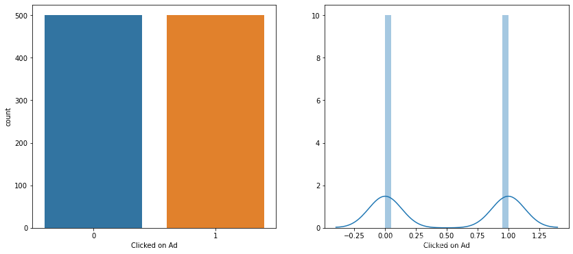
从图中可以看出,点击广告的用户数量与未点击的用户数量相等(即500)。
# joinplot of daily time spent on site and age
sns.jointplot(x='Age', y='Daily Time Spent on Site', data=df)
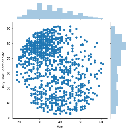
我们可以看到,越来越多的30至40岁的人每天在网站上花费更多的时间。
# Distribution and Relationship Between Variables#creating a pairplot with hue defined by clicked on ad column
sns.pairplot(df, hue='Clicked on Ad', vars=['Daily Time Spent on Site', 'Age', 'Area Income', 'Daily Internet Usage'], palette='husl')
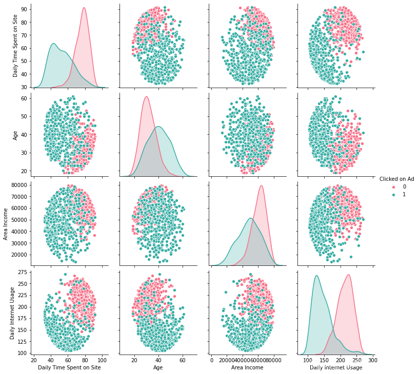
我们可以看到,人们在网站上花费的时间较少,收入较少且年龄相对较大的人倾向于点击广告。
plots = ['Daily Time Spent on Site', 'Age', 'Area Income', 'Daily Internet Usage']
for i in plots:plt.figure(figsize=(14, 6))plt.subplot(1,2,1)sns.boxenplot(df[i])plt.subplot(1,2,2)sns.distplot(df[i], bins=20)plt.title(i)plt.show()
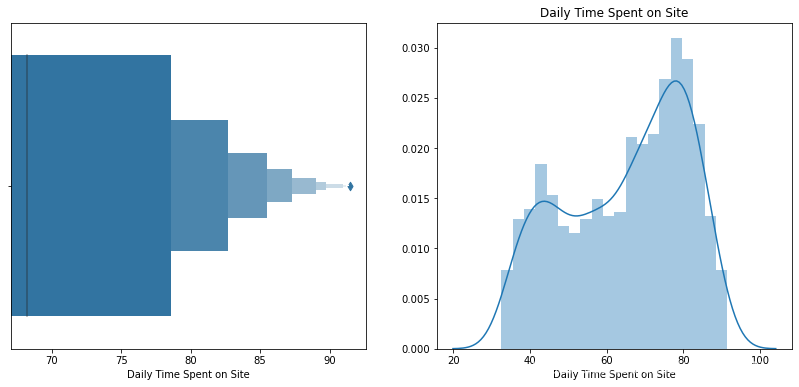
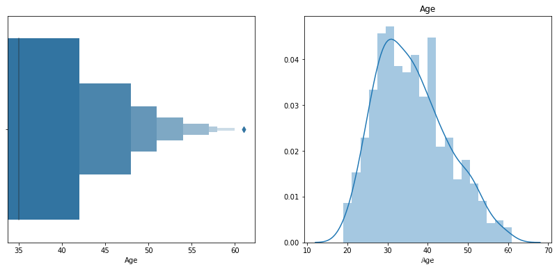
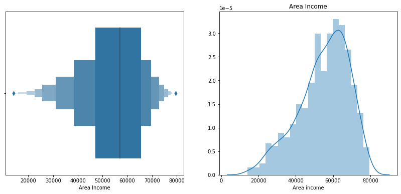
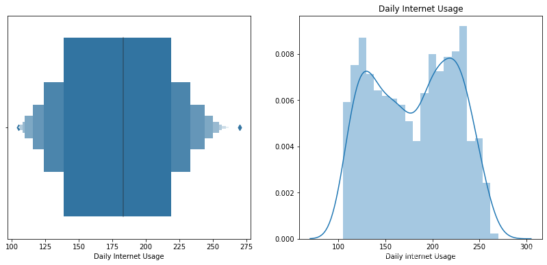
我们可以清楚地看到,网站的日常使用和每天花费的时间有2个高峰(以统计数据为Bi模型)。 这表明我们的数据中存在两个不同的组。 我们不希望用户分布正常,因为有些人会花更多时间在Internet /网站上,而有些人会花更少的时间。
print('oldest person was of: ', df['Age'].max(), 'Years')
print('Youngest person was of: ', df['Age'].min(), 'Years')
print('Average age was of: ', df['Age'].mean(), 'Years')
oldest person was of:  61 Years
Youngest person was of:  19 Years
Average age was of:  36.009 Years
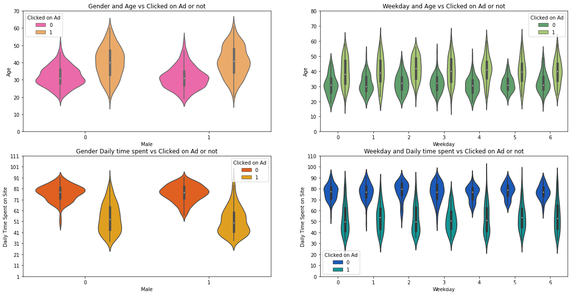
f, ax = plt.subplots(2,2, figsize=(20,10))
sns.violinplot('Male', 'Age', hue='Clicked on Ad', data=df, ax=ax[0, 0], palette='spring')
ax[0,0].set_title('Gender and Age vs Clicked on Ad or not')
ax[0,0].set_yticks(range(0,80,10))sns.violinplot('Weekday', 'Age', hue='Clicked on Ad', data=df, ax=ax[0,1], palette='summer')
ax[0,1].set_title('Weekday and Age vs Clicked on Ad or not')
ax[0,1].set_yticks(range(0,90,10))sns.violinplot('Male', 'Daily Time Spent on Site', hue='Clicked on Ad', data=df, ax=ax[1,0],palette='autumn')
ax[1,0].set_title('Gender Daily time spent vs Clicked on Ad or not' )
ax[1,0].set_yticks(range(1,120,10))sns.violinplot('Weekday', 'Daily Time Spent on Site', hue='Clicked on Ad', data=df,ax=ax[1,1],palette='winter')
ax[1,1].set_title('Weekday and Daily time spent vs Clicked on Ad or not')
ax[1,1].set_yticks(range(0,120,10))
plt.show()
# Correlation Between Variablesfig = plt.figure(figsize=(12,10))
sns.heatmap(df.corr(), cmap='Blues', annot=True)
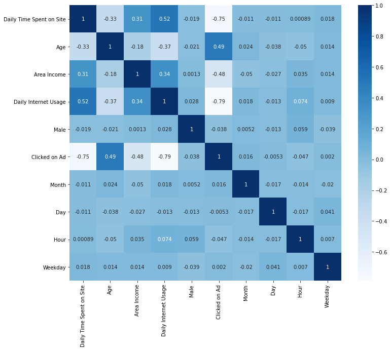
热图使我们可以更好地了解每个功能之间的关系。 相关性在-1和1之间测量。绝对值越高,变量之间的相关度越高。 我们希望每天的互联网使用量和每天在网站上花费的时间与我们的目标变量更加相关。 同样,我们的解释性变量似乎都没有相关,这表明我们的数据中没有共线性。
# Extracted Features Visualizationsf,ax=plt.subplots(1,2,figsize=(14,5))
df['Month'][df['Clicked on Ad']==1].value_counts().sort_index().plot(ax=ax[0])
ax[0].set_title('Months Vs Clicks')
ax[0].set_ylabel('Count of Clicks')
pd.crosstab(df["Clicked on Ad"], df["Month"]).T.plot(kind = 'bar',ax=ax[1]) #bar是小写
#df.groupby(['Month'])['Clicked on Ad'].sum() # alternative code
plt.tight_layout()
plt.show()
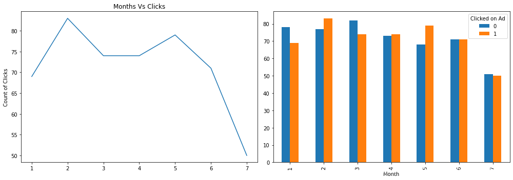
折线图显示了每月的点击次数。 分组条形图显示了7个月内目标变量的分布。 2月点击量最高。
f,ax=plt.subplots(1,2,figsize=(14,5))
pd.crosstab(df['Clicked on Ad'], df['Hour']).T.plot(style=[],ax=ax[0])
pd.pivot_table(df, index=['Weekday'], values=['Clicked on Ad'], aggfunc=np.sum).plot(kind='bar', ax=ax[1])
plt.tight_layout()
plt.show()

此处的线形图表明用户倾向于在一天的晚些时候或清晨点击广告。 根据年龄特征,大多数人都在工作,因此似乎很合适,因为他们早晚都在找时间。 同样,周日点击广告较多。
# Clicked Vs Not Clickeddf.groupby('Clicked on Ad')['Clicked on Ad', 'Daily Time Spent on Site', 'Age','Area Income','Daily Internet Usage'].mean()
| Clicked on Ad | Daily Time Spent on Site | Age | Area Income | Daily Internet Usage | |
|---|---|---|---|---|---|
| Clicked on Ad | |||||
| 0 | 0.0 | 76.85462 | 31.684 | 61385.58642 | 214.51374 |
| 1 | 1.0 | 53.14578 | 40.334 | 48614.41374 | 145.48646 |
df.groupby(['Male', 'Clicked on Ad'])['Clicked on Ad'].count().unstack()
| Clicked on Ad | 0 | 1 |
|---|---|---|
| Male | ||
| 0 | 250 | 269 |
| 1 | 250 | 231 |
hdf = pd.pivot_table(df, index=['Hour'], columns=['Male'], values=['Clicked on Ad'],aggfunc=np.sum).rename(columns={'Clicked on Ad': 'Clicked'}) #透视表
cm = sns.light_palette('green', as_cmap=True) #调色盘
hdf.style.background_gradient(cmap=cm)

每小时和性别分布。 总体而言,女性点击广告的频率高于男性。
f,ax=plt.subplots(1,2,figsize=(14,5))
sns.set_style('whitegrid')
sns.countplot(x='Male', hue='Clicked on Ad', data=df, palette='bwr',ax=ax[0])# overall distribution of males and females count
table=pd.crosstab(df['Weekday'], df['Clicked on Ad']) #交叉表,统计分组频率
table.div(table.sum(1).astype(float), axis=0).plot(kind='bar', stacked=True, ax=ax[1],grid=False)
ax[1].set_title('Stacked Bar Chart of Weekday vs Clicked')
ax[1].set_ylabel('Proportion by Day')
ax[1].set_xlabel('Weekday')
plt.tight_layout() #自动调整子图参数,使之填充整个图像区域
plt.show()
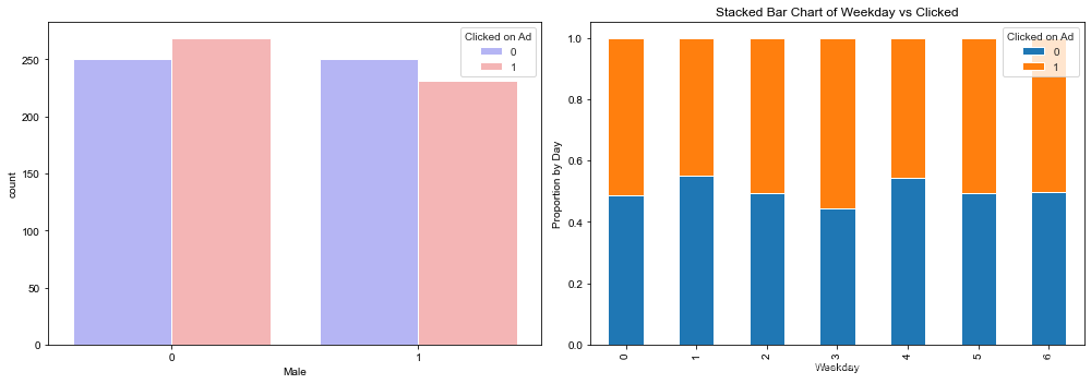
从堆积的条形图看来,如果是星期三,则用户点击广告的机会更大!
sns.factorplot(x='Weekday', y='Age', col='Clicked on Ad', data=df, kind='box',size=5,aspect=2.0)
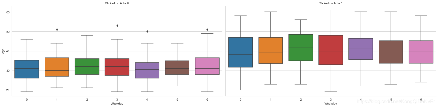
按年龄和工作日比较是否点击过广告的用户。 显然,年龄较大的人倾向于点击广告。
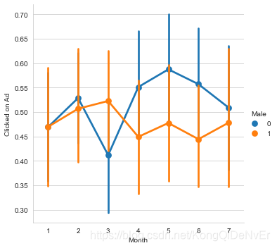
sns.factorplot('Month', 'Clicked on Ad', hue='Male', data=df)
plt.show()
# Identifying Potential Outliers using IQRfor i in numeric_cols:stat= df[i].describe()print(stat)IQR = stat['75%'] - stat['25%']upper = stat['75%']+1.5*IQRlower=stat['25%']-1.5*IQRprint('The upper and lower bounds for suspected outliers are {} and {}.'.format(upper, lower))count 1000.000000
mean 65.000200
std 15.853615
min 32.600000
25% 51.360000
50% 68.215000
75% 78.547500
max 91.430000
Name: Daily Time Spent on Site, dtype: float64
The upper and lower bounds for suspected outliers are 119.32875 and 10.57875.
count 1000.000000
mean 36.009000
std 8.785562
min 19.000000
25% 29.000000
50% 35.000000
75% 42.000000
max 61.000000
Name: Age, dtype: float64
The upper and lower bounds for suspected outliers are 61.5 and 9.5.
count 1000.000000
mean 55000.000080
std 13414.634022
min 13996.500000
25% 47031.802500
50% 57012.300000
75% 65470.635000
max 79484.800000
Name: Area Income, dtype: float64
The upper and lower bounds for suspected outliers are 93128.88375000001 and 19373.553749999992.
count 1000.000000
mean 180.000100
std 43.902339
min 104.780000
25% 138.830000
50% 183.130000
75% 218.792500
max 269.960000
Name: Daily Internet Usage, dtype: float64
The upper and lower bounds for suspected outliers are 338.73625000000004 and 18.886250000000004.
# Basic model building based on the actual data# Importing train_test_split from sklearn.model_selection family
from sklearn.model_selection import train_test_split
# Assigning Numerical columns to X & y only as model can only take numbers
X = df[['Daily Time Spent on Site', 'Age', 'Area Income', 'Daily Internet Usage', 'Male']]
y = df['Clicked on Ad']
# Splitting the data into train & test sets
# test_size is % of data that we want to allocate & random_state ensures a specific set of random splits on our data because
#this train test split is going to occur randomly
X_train, X_test, y_train, y_test = train_test_split(X, y, test_size=0.33, random_state=42)
print(X_train.shape, y_train.shape)
print(X_test.shape, y_test.shape)
(670, 5) (670,)
(330, 5) (330,)
# Building a Basic Model# Import LogisticRegression from sklearn.linear_model family
from sklearn.linear_model import LogisticRegression
#Creating a linear regression object
logreg = LogisticRegression()
# Fit the model on training data using a fit method
model = logreg.fit(X_train, y_train)
model
LogisticRegression(C=1.0, class_weight=None, dual=False, fit_intercept=True,intercept_scaling=1, l1_ratio=None, max_iter=100,multi_class='auto', n_jobs=None, penalty='l2',random_state=None, solver='lbfgs', tol=0.0001, verbose=0,warm_start=False)
# Predictions# The predict method just takes X_test as a parameter, which means it just takes the features to draw predictions
predictions = logreg.predict(X_test)
# Below are the results of predicted click on Ads
predictions[0:20]
array([0, 1, 1, 1, 0, 0, 0, 1, 0, 1, 0, 1, 1, 0, 1, 1, 1, 1, 0, 1],dtype=int64)
# Performance Metrics# Importing classification_report from sklearn.metrics family
from sklearn.metrics import classification_report# Printing classification_report to see the results
print(classification_report(y_test, predictions))
              precision    recall  f1-score   support0       0.86      0.96      0.91       1621       0.96      0.85      0.90       168accuracy                           0.91       330macro avg       0.91      0.91      0.91       330
weighted avg       0.91      0.91      0.91       330
# Importing a pure confusion matrix from sklearn.metrics family
from sklearn.metrics import confusion_matrix# Printing the confusion_matrix
print(confusion_matrix(y_test, predictions))
[[156 6][ 25 143]]
# Feature Engineeringnew_df = df.copy() # just to keep the original dataframe unchanged
# creating pairplot to check effect of datetime variable on target variable
pp = sns.pairplot(new_df, hue= 'Clicked on Ad', vars = ['Month', 'Day', 'Hour', 'Weekday'], palette= 'husl')
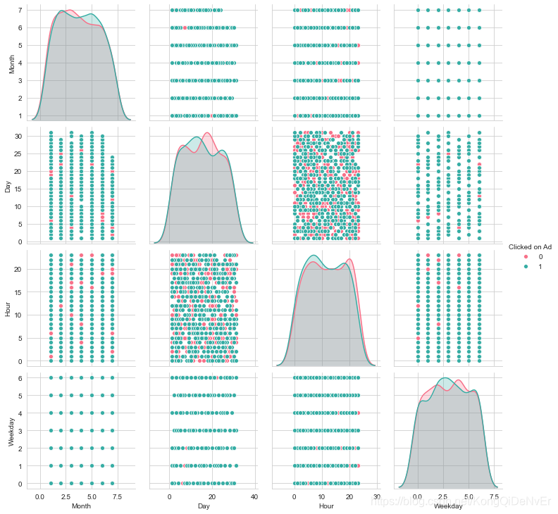
月,日,工作日和小时对目标变量没有任何影响。
# Dummy encoding on Month column
new_df=pd.concat([new_df, pd.get_dummies(new_df['Month'], prefix='Month')], axis=1)
#dummy enconding on weekly column
new_df=pd.concat([new_df, pd.get_dummies(new_df['Weekday'], prefix='Weekday')], axis=1)
#creating buckets for hour columns based on EDA part
new_df['Hour_bins']=pd.cut(new_df['Hour'], bins=[0, 5, 11, 17, 23], labels=['Hour_0-5', 'Hour_6-11','Hour_12-17','Hour_18-23'],include_lowest=True )
# dummy encoding on Hour_bins column
new_df=pd.concat([new_df, pd.get_dummies(new_df['Hour_bins'], prefix='Hour')], axis=1)
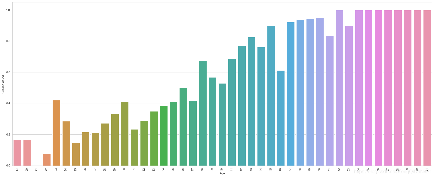
# feature engineering on Age column
plt.figure(figsize=(25,10))
sns.barplot(new_df['Age'], df['Clicked on Ad'], ci=None)
plt.xticks(rotation=90)
(array([ 0, 1, 2, 3, 4, 5, 6, 7, 8, 9, 10, 11, 12, 13, 14, 15, 16,17, 18, 19, 20, 21, 22, 23, 24, 25, 26, 27, 28, 29, 30, 31, 32, 33,34, 35, 36, 37, 38, 39, 40, 41, 42]),[Text(0, 0, '19'),Text(1, 0, '20'),Text(2, 0, '21'),Text(3, 0, '22'),Text(4, 0, '23'),Text(5, 0, '24'),Text(6, 0, '25'),Text(7, 0, '26'),Text(8, 0, '27'),Text(9, 0, '28'),Text(10, 0, '29'),Text(11, 0, '30'),Text(12, 0, '31'),Text(13, 0, '32'),Text(14, 0, '33'),Text(15, 0, '34'),Text(16, 0, '35'),Text(17, 0, '36'),Text(18, 0, '37'),Text(19, 0, '38'),Text(20, 0, '39'),Text(21, 0, '40'),Text(22, 0, '41'),Text(23, 0, '42'),Text(24, 0, '43'),Text(25, 0, '44'),Text(26, 0, '45'),Text(27, 0, '46'),Text(28, 0, '47'),Text(29, 0, '48'),Text(30, 0, '49'),Text(31, 0, '50'),Text(32, 0, '51'),Text(33, 0, '52'),Text(34, 0, '53'),Text(35, 0, '54'),Text(36, 0, '55'),Text(37, 0, '56'),Text(38, 0, '57'),Text(39, 0, '58'),Text(40, 0, '59'),Text(41, 0, '60'),Text(42, 0, '61')])
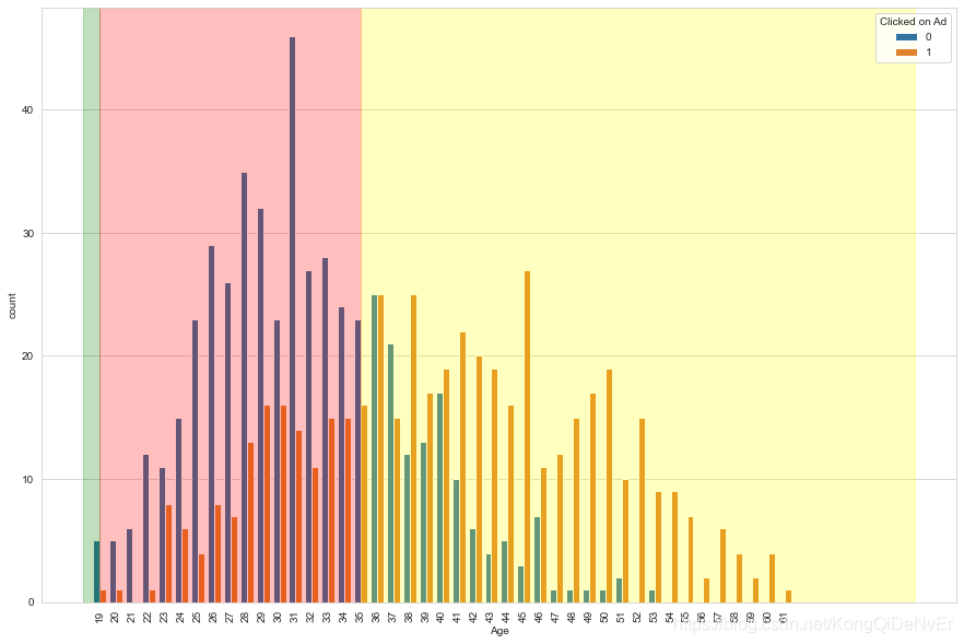
# checking bins
limit_1 = 18
limit_2 = 35x_limit_1 = np.size(df[df['Age']<limit_1]['Age'].unique())
x_limit_2 = np.size(df[df['Age']<limit_2]['Age'].unique())plt.figure(figsize=(15,10))
sns.countplot('Age', hue='Clicked on Ad', data=df)
plt.axvspan(-1, x_limit_1, alpha=0.25, color='green')
plt.axvspan(x_limit_1, x_limit_2, alpha=0.25, color='red')
plt.axvspan(x_limit_2, 50, alpha=0.25, color='yellow')
plt.xticks(rotation=90)
(array([ 0, 1, 2, 3, 4, 5, 6, 7, 8, 9, 10, 11, 12, 13, 14, 15, 16,17, 18, 19, 20, 21, 22, 23, 24, 25, 26, 27, 28, 29, 30, 31, 32, 33,34, 35, 36, 37, 38, 39, 40, 41, 42]),[Text(0, 0, '19'),Text(1, 0, '20'),Text(2, 0, '21'),Text(3, 0, '22'),Text(4, 0, '23'),Text(5, 0, '24'),Text(6, 0, '25'),Text(7, 0, '26'),Text(8, 0, '27'),Text(9, 0, '28'),Text(10, 0, '29'),Text(11, 0, '30'),Text(12, 0, '31'),Text(13, 0, '32'),Text(14, 0, '33'),Text(15, 0, '34'),Text(16, 0, '35'),Text(17, 0, '36'),Text(18, 0, '37'),Text(19, 0, '38'),Text(20, 0, '39'),Text(21, 0, '40'),Text(22, 0, '41'),Text(23, 0, '42'),Text(24, 0, '43'),Text(25, 0, '44'),Text(26, 0, '45'),Text(27, 0, '46'),Text(28, 0, '47'),Text(29, 0, '48'),Text(30, 0, '49'),Text(31, 0, '50'),Text(32, 0, '51'),Text(33, 0, '52'),Text(34, 0, '53'),Text(35, 0, '54'),Text(36, 0, '55'),Text(37, 0, '56'),Text(38, 0, '57'),Text(39, 0, '58'),Text(40, 0, '59'),Text(41, 0, '60'),Text(42, 0, '61')])
# creating bins on Age colummn based on above plots
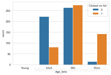
new_df['Age_bins']=pd.cut(new_df['Age'], bins=[0, 18, 30, 45, 70], labels=['Young', 'Adult', 'Mid', 'Elder'])
# verifying the bins by checking the count
sns.countplot('Age_bins', hue='Clicked on Ad', data=new_df)
# dummy enconding on Age column
new_df=pd.concat([new_df, pd.get_dummies(new_df['Age_bins'], prefix='Age')], axis=1)
# dummy encoding on Contry column based on EDA
new_df=pd.concat([new_df, pd.get_dummies(new_df['Country'], prefix='Country')], axis=1)
# Remove redundant and no predictive power features
new_df.drop(['Country', 'Ad Topic Line', 'City', 'Day', 'Month', 'Weekday', 'Hour', 'Hour_bins', 'Age', 'Age_bins'], axis = 1, inplace = True)
new_df.to_csv('new.csv')
new_df.head() # Checking the final dataframe| Daily Time Spent on Site | Area Income | Daily Internet Usage | Male | Clicked on Ad | Month_1 | Month_2 | Month_3 | Month_4 | Month_5 | ... | Country_Uruguay | Country_Uzbekistan | Country_Vanuatu | Country_Venezuela | Country_Vietnam | Country_Wallis and Futuna | Country_Western Sahara | Country_Yemen | Country_Zambia | Country_Zimbabwe | |
|---|---|---|---|---|---|---|---|---|---|---|---|---|---|---|---|---|---|---|---|---|---|
| 0 | 68.95 | 61833.90 | 256.09 | 0 | 0 | 0 | 0 | 1 | 0 | 0 | ... | 0 | 0 | 0 | 0 | 0 | 0 | 0 | 0 | 0 | 0 |
| 1 | 80.23 | 68441.85 | 193.77 | 1 | 0 | 0 | 0 | 0 | 1 | 0 | ... | 0 | 0 | 0 | 0 | 0 | 0 | 0 | 0 | 0 | 0 |
| 2 | 69.47 | 59785.94 | 236.50 | 0 | 0 | 0 | 0 | 1 | 0 | 0 | ... | 0 | 0 | 0 | 0 | 0 | 0 | 0 | 0 | 0 | 0 |
| 3 | 74.15 | 54806.18 | 245.89 | 1 | 0 | 1 | 0 | 0 | 0 | 0 | ... | 0 | 0 | 0 | 0 | 0 | 0 | 0 | 0 | 0 | 0 |
| 4 | 68.37 | 73889.99 | 225.58 | 0 | 0 | 0 | 0 | 0 | 0 | 0 | ... | 0 | 0 | 0 | 0 | 0 | 0 | 0 | 0 | 0 | 0 |
5 rows × 278 columns
# Building Logistic Regression ModelX = new_df.drop(['Clicked on Ad'],1)
y = new_df['Clicked on Ad']
X_train, X_test, y_train, y_test = train_test_split(X, y, test_size=0.20, random_state=42)
# Standarizing the features
from  sklearn.preprocessing  import StandardScaler
stdsc = StandardScaler()
X_train_std = stdsc.fit_transform(X_train)
X_test_std = stdsc.transform(X_test)
print(X_train.shape, y_train.shape)
print(X_test.shape, y_test.shape)
(800, 277) (800,)
(200, 277) (200,)
import statsmodels.api as sm
from scipy import statsX2 = sm.add_constant(X_train_std)
est = sm.OLS(y_train, X2)
est2 = est.fit()
print(est2.summary())
OLS Regression Results
==============================================================================
Dep. Variable: Clicked on Ad R-squared: 0.893
Model: OLS Adj. R-squared: 0.843
Method: Least Squares F-statistic: 17.75
Date: Sun, 09 Aug 2020 Prob (F-statistic): 8.68e-164
Time: 02:03:52 Log-Likelihood: 314.62
No. Observations: 800 AIC: -115.2
Df Residuals: 543 BIC: 1089.
Df Model: 256
Covariance Type: nonrobust
==============================================================================coef std err t P>|t| [0.025 0.975]
------------------------------------------------------------------------------
const 0.4863 0.007 69.390 0.000 0.472 0.500
x1 -0.1816 0.010 -17.728 0.000 -0.202 -0.161
x2 -0.0932 0.009 -10.275 0.000 -0.111 -0.075
x3 -0.2588 0.011 -24.497 0.000 -0.280 -0.238
x4 -0.0166 0.008 -1.974 0.049 -0.033 -8.27e-05
x5 -0.0020 0.002 -0.818 0.414 -0.007 0.003
x6 0.0023 0.002 0.957 0.339 -0.002 0.007
x7 -0.0045 0.002 -1.864 0.063 -0.009 0.000
x8 0.0003 0.002 0.115 0.908 -0.004 0.005
x9 0.0032 0.002 1.296 0.195 -0.002 0.008
x10 -0.0031 0.002 -1.280 0.201 -0.008 0.002
x11 0.0043 0.003 1.694 0.091 -0.001 0.009
x12 -0.0020 0.002 -0.818 0.414 -0.007 0.003
x13 0.0023 0.002 0.957 0.339 -0.002 0.007
x14 -0.0045 0.002 -1.864 0.063 -0.009 0.000
x15 0.0003 0.002 0.115 0.908 -0.004 0.005
x16 0.0032 0.002 1.296 0.195 -0.002 0.008
x17 -0.0031 0.002 -1.280 0.201 -0.008 0.002
x18 0.0043 0.003 1.694 0.091 -0.001 0.009
x19 -0.0020 0.002 -0.818 0.414 -0.007 0.003
x20 0.0023 0.002 0.957 0.339 -0.002 0.007
x21 -0.0045 0.002 -1.864 0.063 -0.009 0.000
x22 0.0003 0.002 0.115 0.908 -0.004 0.005
x23 0.0032 0.002 1.296 0.195 -0.002 0.008
x24 -0.0031 0.002 -1.280 0.201 -0.008 0.002
x25 0.0043 0.003 1.694 0.091 -0.001 0.009
x26 0.0025 0.007 0.339 0.735 -0.012 0.017
x27 -0.0040 0.007 -0.542 0.588 -0.018 0.010
x28 -0.0028 0.007 -0.391 0.696 -0.017 0.011
x29 -0.0011 0.007 -0.150 0.881 -0.015 0.013
x30 -0.0045 0.007 -0.607 0.544 -0.019 0.010
x31 -0.0007 0.008 -0.087 0.930 -0.016 0.014
x32 0.0100 0.007 1.383 0.167 -0.004 0.024
x33 -0.0002 0.006 -0.028 0.978 -0.013 0.013
x34 0.0027 0.006 0.434 0.665 -0.010 0.015
x35 -0.0084 0.006 -1.307 0.192 -0.021 0.004
x36 0.0057 0.006 0.892 0.373 -0.007 0.018
x37 8.946e-19 9.61e-18 0.093 0.926 -1.8e-17 1.98e-17
x38 -0.0305 0.006 -5.329 0.000 -0.042 -0.019
x39 0.0052 0.005 1.066 0.287 -0.004 0.015
x40 0.0316 0.007 4.543 0.000 0.018 0.045
x41 -0.0042 0.007 -0.599 0.550 -0.018 0.010
x42 0.0036 0.007 0.506 0.613 -0.010 0.017
x43 0.0055 0.007 0.775 0.438 -0.008 0.020
x44 0.0010 0.007 0.138 0.891 -0.013 0.015
x45 0.0132 0.007 1.848 0.065 -0.001 0.027
x46 -0.0128 0.007 -1.802 0.072 -0.027 0.001
x47 0.0025 0.007 0.346 0.729 -0.012 0.017
x48 -0.0026 0.007 -0.359 0.720 -0.017 0.011
x49 0.0036 0.007 0.512 0.609 -0.010 0.018
x50 -0.0014 0.007 -0.194 0.846 -0.015 0.013
x51 -0.0055 0.007 -0.771 0.441 -0.019 0.008
x52 -0.0013 0.007 -0.188 0.851 -0.015 0.013
x53 0.0195 0.007 2.745 0.006 0.006 0.033
x54 -0.0066 0.007 -0.926 0.355 -0.021 0.007
x55 -8.59e-05 0.007 -0.012 0.990 -0.014 0.014
x56 -0.0008 0.007 -0.110 0.913 -0.015 0.013
x57 -0.0020 0.007 -0.281 0.779 -0.016 0.012
x58 -0.0056 0.007 -0.788 0.431 -0.020 0.008
x59 -0.0031 0.007 -0.431 0.666 -0.017 0.011
x60 -0.0059 0.007 -0.835 0.404 -0.020 0.008
x61 -0.0078 0.007 -1.105 0.270 -0.022 0.006
x62 -0.0033 0.007 -0.465 0.642 -0.017 0.011
x63 0.0023 0.007 0.329 0.742 -0.012 0.016
x64 0.0029 0.007 0.402 0.688 -0.011 0.017
x65 0.0130 0.007 1.829 0.068 -0.001 0.027
x66 -0.0084 0.007 -1.185 0.237 -0.022 0.006
x67 -0.0021 0.007 -0.294 0.769 -0.016 0.012
x68 -0.0111 0.007 -1.581 0.114 -0.025 0.003
x69 -0.0004 0.007 -0.062 0.950 -0.015 0.014
x70 -0.0058 0.007 -0.806 0.421 -0.020 0.008
x71 -0.0036 0.007 -0.505 0.613 -0.018 0.010
x72 -0.0042 0.007 -0.595 0.552 -0.018 0.010
x73 0.0053 0.007 0.743 0.458 -0.009 0.019
x74 0.0104 0.007 1.465 0.144 -0.004 0.024
x75 -0.0079 0.007 -1.120 0.263 -0.022 0.006
x76 -0.0031 0.007 -0.449 0.653 -0.017 0.011
x77 0.0008 0.007 0.106 0.915 -0.013 0.015
x78 0.0010 0.007 0.136 0.892 -0.013 0.015
x79 -0.0065 0.007 -0.912 0.362 -0.020 0.007
x80 0.0283 0.007 4.009 0.000 0.014 0.042
x81 5.668e-18 1.02e-17 0.555 0.579 -1.44e-17 2.57e-17
x82 0.0065 0.007 0.922 0.357 -0.007 0.020
x83 -0.0039 0.007 -0.545 0.586 -0.018 0.010
x84 -0.0082 0.007 -1.152 0.250 -0.022 0.006
x85 0.0191 0.007 2.701 0.007 0.005 0.033
x86 -0.0035 0.007 -0.488 0.625 -0.017 0.011
x87 -0.0046 0.007 -0.639 0.523 -0.019 0.009
x88 0.0002 0.007 0.024 0.981 -0.014 0.014
x89 -0.0038 0.007 -0.533 0.594 -0.018 0.010
x90 -0.0040 0.007 -0.563 0.573 -0.018 0.010
x91 -0.0069 0.007 -0.971 0.332 -0.021 0.007
x92 -0.0062 0.007 -0.866 0.387 -0.020 0.008
x93 0.0230 0.007 3.188 0.002 0.009 0.037
x94 -0.0169 0.007 -2.369 0.018 -0.031 -0.003
x95 -0.0101 0.007 -1.428 0.154 -0.024 0.004
x96 0.0014 0.007 0.196 0.845 -0.013 0.015
x97 -0.0042 0.007 -0.586 0.558 -0.018 0.010
x98 0.0055 0.007 0.783 0.434 -0.008 0.019
x99 0.0030 0.007 0.425 0.671 -0.011 0.017
x100 -0.0009 0.007 -0.124 0.901 -0.015 0.013
x101 0.0045 0.007 0.635 0.526 -0.009 0.018
x102 0.0069 0.007 0.978 0.329 -0.007 0.021
x103 -0.0028 0.007 -0.391 0.696 -0.017 0.011
x104 -0.0036 0.007 -0.506 0.613 -0.018 0.010
x105 -0.0016 0.007 -0.228 0.820 -0.016 0.012
x106 0.0021 0.007 0.298 0.766 -0.012 0.016
x107 0.0028 0.007 0.390 0.696 -0.011 0.017
x108 0.0003 0.007 0.046 0.963 -0.014 0.014
x109 -0.0100 0.007 -1.406 0.160 -0.024 0.004
x110 0.0002 0.007 0.029 0.977 -0.014 0.014
x111 -0.0054 0.007 -0.762 0.446 -0.019 0.009
x112 0.0004 0.007 0.050 0.961 -0.014 0.014
x113 -0.0061 0.007 -0.863 0.389 -0.020 0.008
x114 -0.0029 0.007 -0.403 0.687 -0.017 0.011
x115 -0.0097 0.007 -1.370 0.171 -0.024 0.004
x116 0.0054 0.007 0.755 0.451 -0.009 0.019
x117 -0.0068 0.007 -0.956 0.339 -0.021 0.007
x118 0.0195 0.007 2.712 0.007 0.005 0.034
x119 -0.0189 0.007 -2.640 0.009 -0.033 -0.005
x120 -0.0113 0.007 -1.585 0.113 -0.025 0.003
x121 -0.0067 0.007 -0.947 0.344 -0.020 0.007
x122 -0.0059 0.007 -0.828 0.408 -0.020 0.008
x123 -0.0095 0.007 -1.346 0.179 -0.023 0.004
x124 0.0089 0.007 1.242 0.215 -0.005 0.023
x125 -0.0013 0.007 -0.189 0.850 -0.015 0.013
x126 0.0138 0.007 1.949 0.052 -0.000 0.028
x127 -0.0049 0.007 -0.687 0.492 -0.019 0.009
x128 -0.0014 0.007 -0.200 0.841 -0.015 0.013
x129 0.0070 0.007 0.980 0.327 -0.007 0.021
x130 -0.0066 0.007 -0.934 0.351 -0.021 0.007
x131 0.0085 0.007 1.203 0.230 -0.005 0.022
x132 8.763e-07 0.007 0.000 1.000 -0.014 0.014
x133 0.0015 0.007 0.217 0.828 -0.012 0.015
x134 -0.0035 0.007 -0.498 0.619 -0.017 0.010
x135 -0.0026 0.007 -0.367 0.713 -0.017 0.011
x136 0.0230 0.007 3.212 0.001 0.009 0.037
x137 -0.0062 0.007 -0.884 0.377 -0.020 0.008
x138 0.0021 0.007 0.298 0.766 -0.012 0.016
x139 0.0039 0.007 0.540 0.589 -0.010 0.018
x140 -0.0010 0.007 -0.140 0.889 -0.015 0.013
x141 -0.0068 0.007 -0.952 0.342 -0.021 0.007
x142 -0.0020 0.007 -0.287 0.774 -0.016 0.012
x143 0.0114 0.007 1.608 0.108 -0.003 0.025
x144 -0.0041 0.007 -0.577 0.564 -0.018 0.010
x145 -0.0012 0.007 -0.169 0.866 -0.015 0.013
x146 0.0125 0.007 1.752 0.080 -0.002 0.027
x147 0.0093 0.007 1.305 0.193 -0.005 0.023
x148 -0.0093 0.007 -1.309 0.191 -0.023 0.005
x149 0.0130 0.007 1.825 0.068 -0.001 0.027
x150 -0.0032 0.007 -0.442 0.659 -0.017 0.011
x151 -0.0025 0.007 -0.354 0.724 -0.017 0.011
x152 0.0019 0.007 0.264 0.792 -0.012 0.016
x153 -0.0128 0.007 -1.791 0.074 -0.027 0.001
x154 -0.0030 0.007 -0.418 0.676 -0.017 0.011
x155 -0.0035 0.007 -0.487 0.626 -0.017 0.010
x156 0.0129 0.007 1.818 0.070 -0.001 0.027
x157 -0.0015 0.007 -0.210 0.834 -0.015 0.012
x158 -0.0044 0.007 -0.614 0.539 -0.018 0.010
x159 0.0044 0.007 0.628 0.530 -0.009 0.018
x160 -0.0028 0.007 -0.400 0.690 -0.017 0.011
x161 0.0167 0.007 2.371 0.018 0.003 0.030
x162 -0.0007 0.007 -0.104 0.917 -0.015 0.013
x163 0.0078 0.007 1.087 0.277 -0.006 0.022
x164 -0.0097 0.007 -1.364 0.173 -0.024 0.004
x165 0.0008 0.007 0.110 0.912 -0.013 0.015
x166 -0.0073 0.007 -1.037 0.300 -0.021 0.007
x167 -0.0144 0.007 -1.990 0.047 -0.029 -0.000
x168 0.0013 0.007 0.185 0.853 -0.013 0.015
x169 -0.0004 0.007 -0.060 0.953 -0.014 0.014
x170 -0.0036 0.007 -0.505 0.614 -0.018 0.010
x171 -0.0017 0.007 -0.244 0.808 -0.016 0.012
x172 -0.0043 0.007 -0.606 0.545 -0.018 0.010
x173 0.0121 0.007 1.690 0.092 -0.002 0.026
x174 -0.0046 0.007 -0.652 0.515 -0.019 0.009
x175 -0.0013 0.007 -0.185 0.853 -0.015 0.013
x176 0.0075 0.007 1.046 0.296 -0.007 0.021
x177 -0.0036 0.007 -0.505 0.614 -0.018 0.010
x178 -0.0029 0.007 -0.405 0.686 -0.017 0.011
x179 -0.0034 0.007 -0.473 0.636 -0.017 0.011
x180 0.0018 0.007 0.253 0.800 -0.012 0.016
x181 -0.0042 0.007 -0.595 0.552 -0.018 0.010
x182 0.0095 0.007 1.337 0.182 -0.004 0.024
x183 0.0034 0.007 0.472 0.637 -0.011 0.017
x184 0.0060 0.007 0.835 0.404 -0.008 0.020
x185 0.0038 0.007 0.529 0.597 -0.010 0.018
x186 -0.0067 0.007 -0.952 0.341 -0.021 0.007
x187 0.0068 0.007 0.951 0.342 -0.007 0.021
x188 0.0004 0.007 0.061 0.951 -0.013 0.014
x189 -0.0026 0.007 -0.368 0.713 -0.017 0.011
x190 0.0060 0.007 0.841 0.401 -0.008 0.020
x191 0.0098 0.007 1.386 0.166 -0.004 0.024
x192 0.0148 0.007 2.076 0.038 0.001 0.029
x193 -0.0101 0.007 -1.424 0.155 -0.024 0.004
x194 -0.0004 0.007 -0.062 0.951 -0.014 0.013
x195 -0.0020 0.007 -0.274 0.784 -0.016 0.012
x196 -0.0024 0.007 -0.338 0.736 -0.016 0.012
x197 -0.0040 0.007 -0.569 0.569 -0.018 0.010
x198 0.0015 0.007 0.212 0.832 -0.012 0.016
x199 -0.0059 0.007 -0.828 0.408 -0.020 0.008
x200 -0.0064 0.007 -0.903 0.367 -0.020 0.008
x201 -0.0113 0.007 -1.595 0.111 -0.025 0.003
x202 -0.0114 0.007 -1.588 0.113 -0.026 0.003
x203 -0.0038 0.007 -0.538 0.591 -0.018 0.010
x204 -0.0001 0.007 -0.018 0.986 -0.014 0.014
x205 0.0018 0.007 0.253 0.800 -0.012 0.016
x206 0.0032 0.007 0.454 0.650 -0.011 0.017
x207 0.0068 0.007 0.962 0.336 -0.007 0.021
x208 0.0003 0.007 0.041 0.967 -0.014 0.014
x209 0.0026 0.007 0.368 0.713 -0.011 0.016
x210 0.0010 0.007 0.142 0.887 -0.013 0.015
x211 0.0011 0.007 0.161 0.872 -0.013 0.015
x212 -0.0057 0.007 -0.801 0.424 -0.020 0.008
x213 -0.0055 0.007 -0.765 0.444 -0.020 0.009
x214 0.0011 0.007 0.157 0.876 -0.013 0.015
x215 0.0013 0.007 0.184 0.854 -0.013 0.015
x216 -0.0069 0.007 -0.969 0.333 -0.021 0.007
x217 0.0050 0.007 0.697 0.486 -0.009 0.019
x218 0.0117 0.007 1.641 0.101 -0.002 0.026
x219 0.0236 0.007 3.309 0.001 0.010 0.038
x220 -0.0012 0.007 -0.170 0.865 -0.015 0.013
x221 0.0002 0.007 0.034 0.973 -0.014 0.014
x222 0.0054 0.007 0.761 0.447 -0.009 0.019
x223 -0.0046 0.007 -0.641 0.522 -0.019 0.009
x224 -0.0064 0.007 -0.908 0.364 -0.020 0.007
x225 -0.0002 0.007 -0.024 0.981 -0.014 0.014
x226 0.0062 0.007 0.869 0.385 -0.008 0.020
x227 0.0054 0.007 0.759 0.448 -0.009 0.019
x228 0.0079 0.007 1.122 0.262 -0.006 0.022
x229 -0.0024 0.007 -0.339 0.735 -0.016 0.012
x230 0.0065 0.007 0.908 0.364 -0.008 0.020
x231 0.0014 0.007 0.196 0.845 -0.013 0.015
x232 -0.0135 0.007 -1.901 0.058 -0.027 0.000
x233 -0.0095 0.007 -1.337 0.182 -0.023 0.004
x234 0.0034 0.007 0.479 0.632 -0.011 0.017
x235 0.0065 0.007 0.908 0.364 -0.008 0.020
x236 0.0146 0.007 2.072 0.039 0.001 0.028
x237 0.0067 0.007 0.950 0.343 -0.007 0.021
x238 0.0165 0.007 2.303 0.022 0.002 0.031
x239 -0.0062 0.007 -0.862 0.389 -0.020 0.008
x240 0.0017 0.007 0.238 0.812 -0.012 0.016
x241 0.0013 0.007 0.181 0.857 -0.013 0.015
x242 0.0064 0.007 0.895 0.371 -0.008 0.020
x243 -0.0061 0.007 -0.850 0.396 -0.020 0.008
x244 -0.0017 0.007 -0.244 0.808 -0.016 0.012
x245 0.0069 0.007 0.977 0.329 -0.007 0.021
x246 -0.0072 0.007 -1.004 0.316 -0.021 0.007
x247 -0.0066 0.007 -0.926 0.355 -0.020 0.007
x248 0.0023 0.007 0.327 0.744 -0.012 0.016
x249 0.0006 0.007 0.080 0.936 -0.013 0.014
x250 -0.0075 0.007 -1.060 0.290 -0.022 0.006
x251 -0.0087 0.007 -1.222 0.222 -0.023 0.005
x252 -0.0098 0.007 -1.374 0.170 -0.024 0.004
x253 0.0040 0.007 0.563 0.574 -0.010 0.018
x254 -0.0015 0.007 -0.207 0.836 -0.015 0.012
x255 -0.0029 0.007 -0.412 0.680 -0.017 0.011
x256 0.0003 0.007 0.037 0.970 -0.014 0.014
x257 0.0075 0.007 1.054 0.292 -0.006 0.021
x258 0.0008 0.007 0.118 0.906 -0.013 0.015
x259 0.0019 0.007 0.264 0.792 -0.012 0.016
x260 -0.0037 0.007 -0.517 0.605 -0.018 0.010
x261 0.0168 0.007 2.379 0.018 0.003 0.031
x262 -0.0033 0.007 -0.472 0.637 -0.017 0.011
x263 0.0130 0.007 1.831 0.068 -0.001 0.027
x264 -0.0047 0.007 -0.666 0.506 -0.019 0.009
x265 0.0032 0.007 0.444 0.657 -0.011 0.017
x266 0.0003 0.007 0.041 0.967 -0.014 0.014
x267 -0.0077 0.007 -1.094 0.274 -0.022 0.006
x268 0.0145 0.007 2.037 0.042 0.001 0.028
x269 0.0046 0.007 0.647 0.518 -0.009 0.019
x270 -0.0067 0.007 -0.938 0.349 -0.021 0.007
x271 -0.0041 0.007 -0.579 0.563 -0.018 0.010
x272 -0.0061 0.007 -0.854 0.393 -0.020 0.008
x273 -0.0067 0.007 -0.948 0.343 -0.021 0.007
x274 -0.0116 0.007 -1.635 0.103 -0.025 0.002
x275 -0.0097 0.007 -1.361 0.174 -0.024 0.004
x276 0.0008 0.007 0.111 0.911 -0.013 0.015
x277 -0.0017 0.007 -0.234 0.815 -0.016 0.012
==============================================================================
Omnibus: 141.574 Durbin-Watson: 1.962
Prob(Omnibus): 0.000 Jarque-Bera (JB): 397.037
Skew: 0.888 Prob(JB): 6.09e-87
Kurtosis: 5.959 Cond. No. 2.76e+16
==============================================================================Warnings:
[1] Standard Errors assume that the covariance matrix of the errors is correctly specified.
[2] The smallest eigenvalue is 4.23e-30. This might indicate that there are
strong multicollinearity problems or that the design matrix is singular.
我们可以看到,特征Male(Gender)对模型没有贡献(即见x4),因此我们实际上可以从模型中删除该变量。 移除变量后,如果“调整后的R平方”与以前的模型相比没有变化。 然后我们可以得出结论,该功能确实对模型没有贡献。
似乎对该模型的有贡献的特征如下:
每天在网站上花费的时间;
每天的Internet使用;
年龄;
国家;
地区收入;
# applying logistic regression model to training data
lr = LogisticRegression(penalty='l2', C=0.1, random_state=42)
lr.fit(X_train_std, y_train)
#predict using model
lr_training_pred = lr.predict(X_train_std)
lr_training_acc = accuracy_score(y_train, lr_training_pred)
print('Accuracy of Logistic regression training set: ', round(lr_training_acc, 3))
Accuracy of Logistic regression training set: 0.992
# creating K fold Cross-validation
from sklearn.model_selection import KFold
kf = KFold(n_splits=10, shuffle=True, random_state=42)
scores = cross_val_score(lr, #modelX_train_std, #feature matrixy_train, #target vectorcv=kf,  #cross-validation techniguescoring='accuracy',  #loss functionn_jobs= -1) # use all cpu scores
print('10 fold CV accuracy: %.3f +/- %.3f' % (np.mean(scores), np.std(scores)))
10 fold CV accuracy: 0.957 +/- 0.018
from sklearn.model_selection import cross_val_predict
print('the cross validated score for Logistic Regression Classifier is: ', round(scores.mean()*100,2))
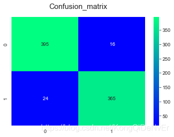
y_pred = cross_val_predict(lr, X_train_std, y_train, cv=10)
sns.heatmap(confusion_matrix(y_train, y_pred), annot=True, fmt='3.0f', cmap='winter')
plt.title('Confusion_matrix', y=1.05, size=15)
the cross validated score for Logistic Regression Classifier is:  95.75
Text(0.5, 1.05, 'Confusion_matrix')
# Random Forest Modelfrom sklearn.ensemble import RandomForestClassifier
rf = RandomForestClassifier(criterion='gini', n_estimators=400,min_samples_split=10, min_samples_leaf=1,max_features='auto', oob_score=True,random_state=42, n_jobs=-1)
rf.fit(X_train_std, y_train)
rf_training_pred = rf.predict(X_train_std)
rf_training_acc = accuracy_score(y_train, rf_training_pred)print('Accuracy of Random Forest training set: ', round(rf_training_acc, 3))
Accuracy of Random Forest training set: 0.994
# creating K fold Cross-validation
kf = KFold(n_splits=10, shuffle=True, random_state=42)
scores = cross_val_score(rf, #modelX_train_std, #Feature matrixy_train, #target vectorcv=kf, #cross-validation techniguescoring='accuracy', #loss functionn_jobs= -1, #use all CPU scores)
print('10 fold CV accuracy: %.3f +/- %.3f' % (np.mean(scores), np.std(scores)))
10 fold CV accuracy: 0.966 +/- 0.011
from sklearn.model_selection import cross_val_predict
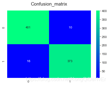
print('the cross validated score for Random Forest Classifier is: ', round(scores.mean()*100,2))
y_pred = cross_val_predict(rf, X_train_std, y_train, cv=10)
sns.heatmap(confusion_matrix(y_train,y_pred),annot=True,fmt='3.0f', cmap='winter')
plt.title('Confusion_matrix', y=1.05, size=15)
the cross validated score for Random Forest Classifier is: 96.62Text(0.5, 1.05, 'Confusion_matrix')
# Test Models Performanceprint('\n\n ---Logistic Regression Model---')
lr_roc_auc = roc_auc_score(y_test, lr.predict(X_test_std))print('Logistic Regression AUC = %2.2f' % lr_roc_auc)
print(classification_report(y_test, lr.predict(X_test_std)))print('\n\n ---Random Forest Model---')
rf_roc_auc = roc_auc_score(y_test, rf.predict(X_test_std))print('Random Forest AUC = %2.2f' % rf_roc_auc)
print(classification_report(y_test, rf.predict(X_test_std)))
 ---Logistic Regression Model---
Logistic Regression AUC = 0.91precision    recall  f1-score   support0       0.84      0.97      0.90        891       0.97      0.86      0.91       111accuracy                           0.91       200macro avg       0.91      0.91      0.90       200
weighted avg       0.91      0.91      0.91       200---Random Forest Model---
Random Forest AUC = 0.93precision    recall  f1-score   support0       0.94      0.90      0.92        891       0.92      0.95      0.94       111accuracy                           0.93       200macro avg       0.93      0.93      0.93       200
weighted avg       0.93      0.93      0.93       200
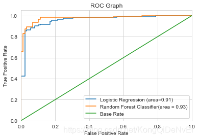
我们可以观察到在测试和训练数据集中,随机森林比逻辑回归模型具有更高的准确性。
# ROC Graph#create ROC Graph
from sklearn.metrics import roc_curve
fpr, tpr, thresholds = roc_curve(y_test, lr.predict_proba(X_test_std)[:,1])
rf_fpr, rf_tpr,rf_thresholds = roc_curve(y_test, rf.predict_proba(X_test_std)[:,1])plt.figure()#Plot Logistic Regression ROC
plt.plot(fpr, tpr, label='Logistic Regression (area=%0.2f)' % lr_roc_auc)#Plot Random Forest ROC
plt.plot(rf_fpr, rf_tpr, label='Random Forest Classifier(area = %0.2f)' % rf_roc_auc)#Plot Base Rate ROC
plt.plot([0,1], [0,1], label='Base Rate')plt.xlim([0.0, 1.0])
plt.ylim([0.0, 1.05])
plt.xlabel('False Positive Rate')
plt.ylabel('True Positive Rate')
plt.title('ROC Graph')
plt.legend(loc='lower right')
plt.show()
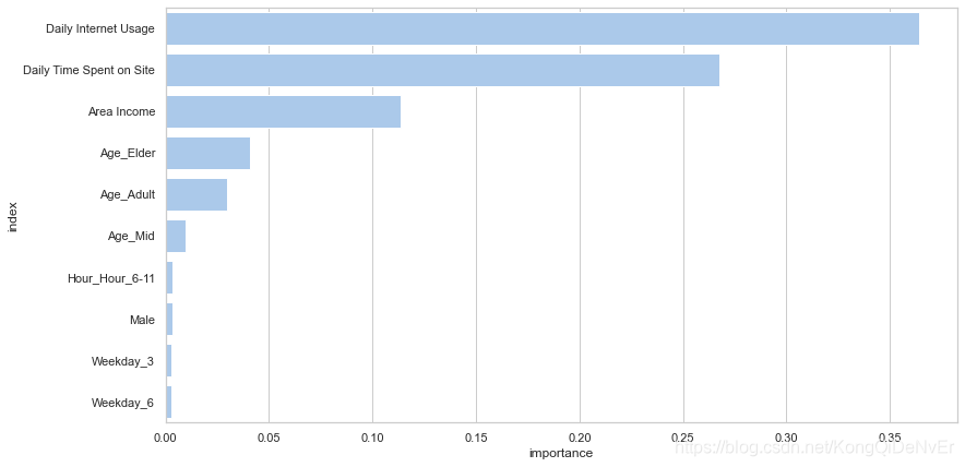
# Random Forest Feature Importancescolumns = X.columns
#converting numpy array list into dataframes
train = pd.DataFrame(np.atleast_2d(X_train_std), columns=columns)
# get feature importance
feature_importances = pd.DataFrame(rf.feature_importances_,index=train.columns,columns=['importance']).sort_values('importance', ascending=False)
feature_importances = feature_importances.reset_index()
feature_importances.head(10)
| index | importance | |
|---|---|---|
| 0 | Daily Internet Usage | 0.364392 |
| 1 | Daily Time Spent on Site | 0.267391 |
| 2 | Area Income | 0.113468 |
| 3 | Age_Elder | 0.041047 |
| 4 | Age_Adult | 0.029649 |
| 5 | Age_Mid | 0.009973 |
| 6 | Hour_Hour_6-11 | 0.003589 |
| 7 | Male | 0.003561 |
| 8 | Weekday_3 | 0.002777 |
| 9 | Weekday_6 | 0.002742 |
sns.set(style='whitegrid')#initialize the matplotlib figure
f, ax = plt.subplots(figsize=(13,7))#plot the feature importance
sns.set_color_codes('pastel')
sns.barplot(x='importance', y='index', data=feature_importances[0:10],label='Total', color='b')
如若内容造成侵权/违法违规/事实不符,请联系编程学习网邮箱:809451989@qq.com进行投诉反馈,一经查实,立即删除!
相关文章
- Linux学习—复习磁盘管理
Linux磁盘管理好坏直接关系到整个系统性能问题 df:列出文件系统的整体磁盘使用量 -a :列出所有的文件系统,包括系统特有的 /proc 等文件系统; -k :以 KBytes 的容量显示各文件系统; -m :以 MBytes 的容量显示各文件系统; -h :以人们较易阅读的 GBytes, MBytes, KBytes…...
2024/4/29 7:05:41 - 【扩欧】同余方程
SampleSampleSample InputInputInput 3 10SampleSampleSample OutputOutputOutput 7HintHintHint 扩展欧几里得 (第一个题解的解释个人觉得比较好) #include<algorithm> #include<iostream> #include<cstring> #include<cstdio> #define ll long lon…...
2024/4/29 7:05:35 - 湖南大学ACM程序设计新生杯大赛(同步赛)(重现赛)
比赛地址传送口 A.Array ps:待补 Array题解 B.Build ps:待补 Build题解 C.Do you like banana? 计算几何 题意:判断线段是否相交 思路:向量叉乘 线段相交判定知识点参考 ac代码: #include<iostream> #include<cstdio> #define ZERO 1e-9using namespace …...
2024/4/30 2:35:44 - [纸上谈兵]Web服务器机制
目录通信协议Http协议HTTPS协议套接字协议服务器模型本文从通信协议、套接字通信(Socket)、Web服务模型三个方面了解Web服务器机制 web服务器就是指类tomcat服务器通信协议Http协议http是请求/响应模型, 一个浏览器的http请求/响应的流程大概可以用以下4步表示 1、客户端浏览器…...
2024/4/29 7:05:31 - String字符串练习题
String字符串练习题 1、下面代码的运行结果为 public class A {public String str = new String("hello");public char[] ch = {t,e,s,t};public void change(String str, char ch[]){str = "hello world";ch[0] = b;}public static void main(String[] ar…...
2024/4/29 7:05:37 - Spring框架学习---Spring的IoC高级特性之BeanFactory和FactoryBean
Spring框架学习—Spring的IoC高级特性之BeanFactory和FactoryBean BeanFactory和FactoryBeanBeanFactory接⼝是容器的顶级接⼝,定义了容器的⼀些基础⾏为,负责⽣产和管理Bean的⼀个⼯⼚,具体使⽤它下⾯的⼦接⼝类型,⽐如ApplicationContext; Spring中Bean有两种,⼀种是普…...
2024/4/30 21:55:15 - SuperMap 栅格数据空间分析(二)
我们接着上次的栅格数据空间分析的讲,上次说了三维晕渲图原理和正射三维影像原理,上次还没说完,现在接着讲。 表面距离、面积和体积原理—表面距离用来计算栅格表面距离,即计算在栅格数据集拟合的三维曲面上沿指定的线段或折线段的曲面距离。表面量算所量算的距离是曲面上的…...
2024/4/29 7:05:17 - 从节税的角度来讲,公司、个体户和个人独资企业哪一个更有优势?
缴税纳税是每个公民的责任和义务,在纳税热同时利用国家税收政策减少税收压力也是很多老板和财务关注的问题。在有实际业务发生的情况下,缺少进项成本导致企业所得税压力增大的情况屡见不鲜,我国税负重一直是让公司老板头疼的问题,25%的企业所得税,20%的分红税,3%、6%、9%…...
2024/4/29 7:05:23 - 最小生成树-Kruskal_Prim算法实现(Javascript实现)
最小生成树 说明这里不会对原理进行详细的分析讲解,只说构建的过程 这里假设所有的图的所有节点都是连通了,不会是非 最小生成树的构建过程最关键的就是对于成环的判断使用的图Kruskal算法 边集合数据结构 //边集合 edges = [] //边集合中元素 function node(start, end, wei…...
2024/4/29 2:52:52 - python之爬虫相关
文章目录1.基础爬虫1.1.请求与返回1.2.response对象的方法1.3.获取翻译的python代码示例1.4.获取图片实例1.5.IP代理1.6.url详解1.7.请求头常见参数1.8.常见响应状态码1.9.常见相关函数1.10.cookie2.更简单的request库的使用3.csv文件3.python连接mysql数据库4.python与mongoDB…...
2024/4/29 2:52:46 - libevent学习之Reactor模式
1.什么是Reactor模式维基百科上说:“The reactor design pattern is an event handling pattern for handling service requests delivered concurrently by one or more inputs. The service handler then demultiplexes the incoming requests and dispatches them synchron…...
2024/4/29 2:52:44 - wordpress主题后台教程(九):多个图片上传表单
节教程需要再上一篇教程的基础上完成,请先准备好上一篇教程中的代码和js文件。本教程要实现的目标是后台能有多个图片上传表单。首先我们修改表单,添加多个上传按钮,还加上显示图片用的div容器。上一篇教程中的js代码中是通过文本域的id值来获取元素的,如果有多个文件上传表…...
2024/4/29 7:05:22 - python简单进阶,Generator
Generator 看完了上一篇python简单进阶,Iteration,再看这一篇。 1、先看看一个比较精简的说明 the differences between Generator function and a Normal function: 1.Generator函数包含一个 yield语句 2.当调用这个函数的时候,并不立即执行,而是返回一个iterator 3. __it…...
2024/4/29 7:05:09 - Improving Question Answering by Commonsense-Based Pre-Training
摘要 尽管神经网络的模型在各种NLP任务上达到很高的效果,但是它们不能够回答那些需要具备常识知识才能回答的问题。我们认为主要原因是缺乏单词概念之间的联系。为了弥补这个缺陷,我们提出一种利用外部语义网ConceptNet的简单模型。我们预训练概念之间直接或间接相连的关系模…...
2024/4/29 4:16:32 - SpringBoot + Thymeleaf调用接口报错EL1007E: Property or field ‘xxx‘ canno be found on null
关键报错信息如下:2020-08-09 18:35:20.334 ERROR 1936 --- [http-nio-8080-exec-1] o.a.c.c.C.[.[.[/].[dispatcherServlet] : Servlet.service() for servlet [dispatcherServlet] in context with path [] threw exception [Request processing failed; nested exceptio…...
2024/4/30 19:58:56 - banner 动画特效 逐渐拉近变大 css
banner 慢慢变大 案例1:https://www.cmseasy.cn/demo/business-template/v451/qi-ta/ 案例2<!DOCTYPE html> <html lang="en"> <head><meta http-equiv="Content-Type" content="text/html; charset=UTF-8"><meta n…...
2024/4/29 7:05:00 - Leetcode 823. 带因子的二叉树 C++
Leetcode 823. 带因子的二叉树 题目 给出一个含有不重复整数元素的数组,每个整数均大于 1。 我们用这些整数来构建二叉树,每个整数可以使用任意次数。 其中:每个非叶结点的值应等于它的两个子结点的值的乘积。 满足条件的二叉树一共有多少个?返回的结果应模除 10 ** 9 + 7。…...
2024/4/29 7:04:55 - 《最好的我们》观后感
也许是年纪大了,真的不适合看这种剧,哭了好多次。 还记得路星河对耿耿的表白: 当路星河堵在厕所门口向耿耿表白,“你干嘛?”,“表白啊,一次不行两次,两次不行三次”。 当路星河离开时向耿耿表白:“我就是喜欢你,没有原因”,“你就让我最后一次说这个吧,因为再不说就…...
2024/4/29 7:05:01 - 程序员轻松绘图神器
我们程序员在工作生活中,有很多场合下需要绘制图表,比如PPT里的图表,学习笔记的一些助记图,还有最常见的,工作中大量使用的流程图。 在 Window 下,我们有很多好用的工具,比如 Visio 、 EA 等等。这些软件也很好用,但都有个缺点,那就是太复杂。我们需要一定的美工基础,…...
2024/4/29 7:04:46 - 小马哥讲Spring核心编程思想 第六周 Spring IoC依赖来源
小马哥讲Spring核心编程思想 第六周 Spring IoC依赖来源 待补充,因时间较紧,后续补充。 01-03 课程介绍,内容综述,课前准备 04丨特性总览:核心特性、数据存储、Web技术、框架整合与测试 05丨Spring版本特性:Spring各个版本引入了哪些新特性? 06丨Spring模块化设计:Spri…...
2024/4/29 7:04:47
最新文章
- 全网最强JavaWeb笔记 | 万字长文爆肝JavaWeb开发——day08数据库Mybatis入门
万字长文爆肝黑马程序员2023最新版JavaWeb教程。这套教程打破常规,不再局限于过时的老套JavaWeb技术,而是与时俱进,运用的都是企业中流行的前沿技术。笔者认真跟着这个教程,再一次认真学习一遍JavaWeb教程,温故而知新&…...
2024/5/2 0:06:35 - 梯度消失和梯度爆炸的一些处理方法
在这里是记录一下梯度消失或梯度爆炸的一些处理技巧。全当学习总结了如有错误还请留言,在此感激不尽。 权重和梯度的更新公式如下: w w − η ⋅ ∇ w w w - \eta \cdot \nabla w ww−η⋅∇w 个人通俗的理解梯度消失就是网络模型在反向求导的时候出…...
2024/3/20 10:50:27 - 前端 js 经典:字符编码详解
前言:计算机只能识别二进制,开发语言中数据类型还有数字,字母,中文,特殊符号等,都需要转化成二进制编码才能让技术机识别。 一. 编码方式 ACSLL、Unicode、utf-8、URL 编码、base64 等。 1. ACSLL 对英语…...
2024/4/29 3:52:58 - 自动化标准Makefile与lds
makefile的自动化,需要使用变量,以及自动变量。 实行命令行与参数的分离。 命令行只与变量打交道,而变量则携带不同的参数,这样,通过修改变量,命令的执行结果不同。 可以简单理解为,命令行是个…...
2024/4/30 2:45:52 - 416. 分割等和子集问题(动态规划)
题目 题解 class Solution:def canPartition(self, nums: List[int]) -> bool:# badcaseif not nums:return True# 不能被2整除if sum(nums) % 2 ! 0:return False# 状态定义:dp[i][j]表示当背包容量为j,用前i个物品是否正好可以将背包填满ÿ…...
2024/5/1 10:25:26 - 【Java】ExcelWriter自适应宽度工具类(支持中文)
工具类 import org.apache.poi.ss.usermodel.Cell; import org.apache.poi.ss.usermodel.CellType; import org.apache.poi.ss.usermodel.Row; import org.apache.poi.ss.usermodel.Sheet;/*** Excel工具类** author xiaoming* date 2023/11/17 10:40*/ public class ExcelUti…...
2024/5/1 13:20:04 - Spring cloud负载均衡@LoadBalanced LoadBalancerClient
LoadBalance vs Ribbon 由于Spring cloud2020之后移除了Ribbon,直接使用Spring Cloud LoadBalancer作为客户端负载均衡组件,我们讨论Spring负载均衡以Spring Cloud2020之后版本为主,学习Spring Cloud LoadBalance,暂不讨论Ribbon…...
2024/5/1 21:18:12 - TSINGSEE青犀AI智能分析+视频监控工业园区周界安全防范方案
一、背景需求分析 在工业产业园、化工园或生产制造园区中,周界防范意义重大,对园区的安全起到重要的作用。常规的安防方式是采用人员巡查,人力投入成本大而且效率低。周界一旦被破坏或入侵,会影响园区人员和资产安全,…...
2024/5/1 4:07:45 - VB.net WebBrowser网页元素抓取分析方法
在用WebBrowser编程实现网页操作自动化时,常要分析网页Html,例如网页在加载数据时,常会显示“系统处理中,请稍候..”,我们需要在数据加载完成后才能继续下一步操作,如何抓取这个信息的网页html元素变化&…...
2024/4/30 23:32:22 - 【Objective-C】Objective-C汇总
方法定义 参考:https://www.yiibai.com/objective_c/objective_c_functions.html Objective-C编程语言中方法定义的一般形式如下 - (return_type) method_name:( argumentType1 )argumentName1 joiningArgument2:( argumentType2 )argumentName2 ... joiningArgu…...
2024/4/30 23:16:16 - 【洛谷算法题】P5713-洛谷团队系统【入门2分支结构】
👨💻博客主页:花无缺 欢迎 点赞👍 收藏⭐ 留言📝 加关注✅! 本文由 花无缺 原创 收录于专栏 【洛谷算法题】 文章目录 【洛谷算法题】P5713-洛谷团队系统【入门2分支结构】🌏题目描述🌏输入格…...
2024/5/1 6:35:25 - 【ES6.0】- 扩展运算符(...)
【ES6.0】- 扩展运算符... 文章目录 【ES6.0】- 扩展运算符...一、概述二、拷贝数组对象三、合并操作四、参数传递五、数组去重六、字符串转字符数组七、NodeList转数组八、解构变量九、打印日志十、总结 一、概述 **扩展运算符(...)**允许一个表达式在期望多个参数࿰…...
2024/5/1 11:24:00 - 摩根看好的前智能硬件头部品牌双11交易数据极度异常!——是模式创新还是饮鸩止渴?
文 | 螳螂观察 作者 | 李燃 双11狂欢已落下帷幕,各大品牌纷纷晒出优异的成绩单,摩根士丹利投资的智能硬件头部品牌凯迪仕也不例外。然而有爆料称,在自媒体平台发布霸榜各大榜单喜讯的凯迪仕智能锁,多个平台数据都表现出极度异常…...
2024/5/1 4:35:02 - Go语言常用命令详解(二)
文章目录 前言常用命令go bug示例参数说明 go doc示例参数说明 go env示例 go fix示例 go fmt示例 go generate示例 总结写在最后 前言 接着上一篇继续介绍Go语言的常用命令 常用命令 以下是一些常用的Go命令,这些命令可以帮助您在Go开发中进行编译、测试、运行和…...
2024/5/1 20:22:59 - 用欧拉路径判断图同构推出reverse合法性:1116T4
http://cplusoj.com/d/senior/p/SS231116D 假设我们要把 a a a 变成 b b b,我们在 a i a_i ai 和 a i 1 a_{i1} ai1 之间连边, b b b 同理,则 a a a 能变成 b b b 的充要条件是两图 A , B A,B A,B 同构。 必要性显然࿰…...
2024/4/30 22:14:26 - 【NGINX--1】基础知识
1、在 Debian/Ubuntu 上安装 NGINX 在 Debian 或 Ubuntu 机器上安装 NGINX 开源版。 更新已配置源的软件包信息,并安装一些有助于配置官方 NGINX 软件包仓库的软件包: apt-get update apt install -y curl gnupg2 ca-certificates lsb-release debian-…...
2024/5/1 6:34:45 - Hive默认分割符、存储格式与数据压缩
目录 1、Hive默认分割符2、Hive存储格式3、Hive数据压缩 1、Hive默认分割符 Hive创建表时指定的行受限(ROW FORMAT)配置标准HQL为: ... ROW FORMAT DELIMITED FIELDS TERMINATED BY \u0001 COLLECTION ITEMS TERMINATED BY , MAP KEYS TERMI…...
2024/5/2 0:07:22 - 【论文阅读】MAG:一种用于航天器遥测数据中有效异常检测的新方法
文章目录 摘要1 引言2 问题描述3 拟议框架4 所提出方法的细节A.数据预处理B.变量相关分析C.MAG模型D.异常分数 5 实验A.数据集和性能指标B.实验设置与平台C.结果和比较 6 结论 摘要 异常检测是保证航天器稳定性的关键。在航天器运行过程中,传感器和控制器产生大量周…...
2024/4/30 20:39:53 - --max-old-space-size=8192报错
vue项目运行时,如果经常运行慢,崩溃停止服务,报如下错误 FATAL ERROR: CALL_AND_RETRY_LAST Allocation failed - JavaScript heap out of memory 因为在 Node 中,通过JavaScript使用内存时只能使用部分内存(64位系统&…...
2024/5/1 4:45:02 - 基于深度学习的恶意软件检测
恶意软件是指恶意软件犯罪者用来感染个人计算机或整个组织的网络的软件。 它利用目标系统漏洞,例如可以被劫持的合法软件(例如浏览器或 Web 应用程序插件)中的错误。 恶意软件渗透可能会造成灾难性的后果,包括数据被盗、勒索或网…...
2024/5/1 8:32:56 - JS原型对象prototype
让我简单的为大家介绍一下原型对象prototype吧! 使用原型实现方法共享 1.构造函数通过原型分配的函数是所有对象所 共享的。 2.JavaScript 规定,每一个构造函数都有一个 prototype 属性,指向另一个对象,所以我们也称为原型对象…...
2024/5/1 14:33:22 - C++中只能有一个实例的单例类
C中只能有一个实例的单例类 前面讨论的 President 类很不错,但存在一个缺陷:无法禁止通过实例化多个对象来创建多名总统: President One, Two, Three; 由于复制构造函数是私有的,其中每个对象都是不可复制的,但您的目…...
2024/5/1 11:51:23 - python django 小程序图书借阅源码
开发工具: PyCharm,mysql5.7,微信开发者工具 技术说明: python django html 小程序 功能介绍: 用户端: 登录注册(含授权登录) 首页显示搜索图书,轮播图࿰…...
2024/5/1 5:23:20 - 电子学会C/C++编程等级考试2022年03月(一级)真题解析
C/C++等级考试(1~8级)全部真题・点这里 第1题:双精度浮点数的输入输出 输入一个双精度浮点数,保留8位小数,输出这个浮点数。 时间限制:1000 内存限制:65536输入 只有一行,一个双精度浮点数。输出 一行,保留8位小数的浮点数。样例输入 3.1415926535798932样例输出 3.1…...
2024/5/1 20:56:20 - 配置失败还原请勿关闭计算机,电脑开机屏幕上面显示,配置失败还原更改 请勿关闭计算机 开不了机 这个问题怎么办...
解析如下:1、长按电脑电源键直至关机,然后再按一次电源健重启电脑,按F8健进入安全模式2、安全模式下进入Windows系统桌面后,按住“winR”打开运行窗口,输入“services.msc”打开服务设置3、在服务界面,选中…...
2022/11/19 21:17:18 - 错误使用 reshape要执行 RESHAPE,请勿更改元素数目。
%读入6幅图像(每一幅图像的大小是564*564) f1 imread(WashingtonDC_Band1_564.tif); subplot(3,2,1),imshow(f1); f2 imread(WashingtonDC_Band2_564.tif); subplot(3,2,2),imshow(f2); f3 imread(WashingtonDC_Band3_564.tif); subplot(3,2,3),imsho…...
2022/11/19 21:17:16 - 配置 已完成 请勿关闭计算机,win7系统关机提示“配置Windows Update已完成30%请勿关闭计算机...
win7系统关机提示“配置Windows Update已完成30%请勿关闭计算机”问题的解决方法在win7系统关机时如果有升级系统的或者其他需要会直接进入一个 等待界面,在等待界面中我们需要等待操作结束才能关机,虽然这比较麻烦,但是对系统进行配置和升级…...
2022/11/19 21:17:15 - 台式电脑显示配置100%请勿关闭计算机,“准备配置windows 请勿关闭计算机”的解决方法...
有不少用户在重装Win7系统或更新系统后会遇到“准备配置windows,请勿关闭计算机”的提示,要过很久才能进入系统,有的用户甚至几个小时也无法进入,下面就教大家这个问题的解决方法。第一种方法:我们首先在左下角的“开始…...
2022/11/19 21:17:14 - win7 正在配置 请勿关闭计算机,怎么办Win7开机显示正在配置Windows Update请勿关机...
置信有很多用户都跟小编一样遇到过这样的问题,电脑时发现开机屏幕显现“正在配置Windows Update,请勿关机”(如下图所示),而且还需求等大约5分钟才干进入系统。这是怎样回事呢?一切都是正常操作的,为什么开时机呈现“正…...
2022/11/19 21:17:13 - 准备配置windows 请勿关闭计算机 蓝屏,Win7开机总是出现提示“配置Windows请勿关机”...
Win7系统开机启动时总是出现“配置Windows请勿关机”的提示,没过几秒后电脑自动重启,每次开机都这样无法进入系统,此时碰到这种现象的用户就可以使用以下5种方法解决问题。方法一:开机按下F8,在出现的Windows高级启动选…...
2022/11/19 21:17:12 - 准备windows请勿关闭计算机要多久,windows10系统提示正在准备windows请勿关闭计算机怎么办...
有不少windows10系统用户反映说碰到这样一个情况,就是电脑提示正在准备windows请勿关闭计算机,碰到这样的问题该怎么解决呢,现在小编就给大家分享一下windows10系统提示正在准备windows请勿关闭计算机的具体第一种方法:1、2、依次…...
2022/11/19 21:17:11 - 配置 已完成 请勿关闭计算机,win7系统关机提示“配置Windows Update已完成30%请勿关闭计算机”的解决方法...
今天和大家分享一下win7系统重装了Win7旗舰版系统后,每次关机的时候桌面上都会显示一个“配置Windows Update的界面,提示请勿关闭计算机”,每次停留好几分钟才能正常关机,导致什么情况引起的呢?出现配置Windows Update…...
2022/11/19 21:17:10 - 电脑桌面一直是清理请关闭计算机,windows7一直卡在清理 请勿关闭计算机-win7清理请勿关机,win7配置更新35%不动...
只能是等着,别无他法。说是卡着如果你看硬盘灯应该在读写。如果从 Win 10 无法正常回滚,只能是考虑备份数据后重装系统了。解决来方案一:管理员运行cmd:net stop WuAuServcd %windir%ren SoftwareDistribution SDoldnet start WuA…...
2022/11/19 21:17:09 - 计算机配置更新不起,电脑提示“配置Windows Update请勿关闭计算机”怎么办?
原标题:电脑提示“配置Windows Update请勿关闭计算机”怎么办?win7系统中在开机与关闭的时候总是显示“配置windows update请勿关闭计算机”相信有不少朋友都曾遇到过一次两次还能忍但经常遇到就叫人感到心烦了遇到这种问题怎么办呢?一般的方…...
2022/11/19 21:17:08 - 计算机正在配置无法关机,关机提示 windows7 正在配置windows 请勿关闭计算机 ,然后等了一晚上也没有关掉。现在电脑无法正常关机...
关机提示 windows7 正在配置windows 请勿关闭计算机 ,然后等了一晚上也没有关掉。现在电脑无法正常关机以下文字资料是由(历史新知网www.lishixinzhi.com)小编为大家搜集整理后发布的内容,让我们赶快一起来看一下吧!关机提示 windows7 正在配…...
2022/11/19 21:17:05 - 钉钉提示请勿通过开发者调试模式_钉钉请勿通过开发者调试模式是真的吗好不好用...
钉钉请勿通过开发者调试模式是真的吗好不好用 更新时间:2020-04-20 22:24:19 浏览次数:729次 区域: 南阳 > 卧龙 列举网提醒您:为保障您的权益,请不要提前支付任何费用! 虚拟位置外设器!!轨迹模拟&虚拟位置外设神器 专业用于:钉钉,外勤365,红圈通,企业微信和…...
2022/11/19 21:17:05 - 配置失败还原请勿关闭计算机怎么办,win7系统出现“配置windows update失败 还原更改 请勿关闭计算机”,长时间没反应,无法进入系统的解决方案...
前几天班里有位学生电脑(windows 7系统)出问题了,具体表现是开机时一直停留在“配置windows update失败 还原更改 请勿关闭计算机”这个界面,长时间没反应,无法进入系统。这个问题原来帮其他同学也解决过,网上搜了不少资料&#x…...
2022/11/19 21:17:04 - 一个电脑无法关闭计算机你应该怎么办,电脑显示“清理请勿关闭计算机”怎么办?...
本文为你提供了3个有效解决电脑显示“清理请勿关闭计算机”问题的方法,并在最后教给你1种保护系统安全的好方法,一起来看看!电脑出现“清理请勿关闭计算机”在Windows 7(SP1)和Windows Server 2008 R2 SP1中,添加了1个新功能在“磁…...
2022/11/19 21:17:03 - 请勿关闭计算机还原更改要多久,电脑显示:配置windows更新失败,正在还原更改,请勿关闭计算机怎么办...
许多用户在长期不使用电脑的时候,开启电脑发现电脑显示:配置windows更新失败,正在还原更改,请勿关闭计算机。。.这要怎么办呢?下面小编就带着大家一起看看吧!如果能够正常进入系统,建议您暂时移…...
2022/11/19 21:17:02 - 还原更改请勿关闭计算机 要多久,配置windows update失败 还原更改 请勿关闭计算机,电脑开机后一直显示以...
配置windows update失败 还原更改 请勿关闭计算机,电脑开机后一直显示以以下文字资料是由(历史新知网www.lishixinzhi.com)小编为大家搜集整理后发布的内容,让我们赶快一起来看一下吧!配置windows update失败 还原更改 请勿关闭计算机&#x…...
2022/11/19 21:17:01 - 电脑配置中请勿关闭计算机怎么办,准备配置windows请勿关闭计算机一直显示怎么办【图解】...
不知道大家有没有遇到过这样的一个问题,就是我们的win7系统在关机的时候,总是喜欢显示“准备配置windows,请勿关机”这样的一个页面,没有什么大碍,但是如果一直等着的话就要两个小时甚至更久都关不了机,非常…...
2022/11/19 21:17:00 - 正在准备配置请勿关闭计算机,正在准备配置windows请勿关闭计算机时间长了解决教程...
当电脑出现正在准备配置windows请勿关闭计算机时,一般是您正对windows进行升级,但是这个要是长时间没有反应,我们不能再傻等下去了。可能是电脑出了别的问题了,来看看教程的说法。正在准备配置windows请勿关闭计算机时间长了方法一…...
2022/11/19 21:16:59 - 配置失败还原请勿关闭计算机,配置Windows Update失败,还原更改请勿关闭计算机...
我们使用电脑的过程中有时会遇到这种情况,当我们打开电脑之后,发现一直停留在一个界面:“配置Windows Update失败,还原更改请勿关闭计算机”,等了许久还是无法进入系统。如果我们遇到此类问题应该如何解决呢࿰…...
2022/11/19 21:16:58 - 如何在iPhone上关闭“请勿打扰”
Apple’s “Do Not Disturb While Driving” is a potentially lifesaving iPhone feature, but it doesn’t always turn on automatically at the appropriate time. For example, you might be a passenger in a moving car, but your iPhone may think you’re the one dri…...
2022/11/19 21:16:57