论文来源:Deep Residual Learning for Image Recognition

Deep Residual Learning for Image Recognition

Kaiming He Xiangyu Zhang Shaoqing Ren Jian Sun Microsoft Research {kahe, v-xiangz, v-shren, jiansun}@microsoft.com

Abstract

Deeper neural networks are more difficult to train. We present a residual learning framework to ease the training of networks that are substantially deeper than those used previously. We explicitly reformulate the layers as learning residual functions with reference to the layer inputs, instead of learning unreferenced functions. We provide comprehensive empirical evidence showing that these residual networks are easier to optimize, and can gain accuracy from considerably increased depth. On the ImageNet dataset we evaluate residual nets with a depth of up to 152 layers—8× deeper than VGG nets [40] but still having lower complexity. An ensemble of these residual nets achieves 3.57% error on the ImageNet test set. This result won the 1st place on the ILSVRC 2015 classification task. We also present analysis on CIFAR-10 with 100 and 1000 layers.
The depth of representations is of central importance for many visual recognition tasks. Solely due to our extremely deep representations, we obtain a 28% relative improvement on the COCO object detection dataset. Deep residual nets are foundations of our submissions to ILSVRC & COCO 2015 competitions , where we also won the 1st places on the tasks of ImageNet detection, ImageNet localization, COCO detection, and COCO segmentation.

摘要

深层次网络的训练往往更加的困难。本文提出了一种residual learning 模块来简化深层网络的训练。Residual模块在输出层参照了输入x，而普通网络是直接输出。大量的实验证明，这些残差网络更易于优化，并能在大幅度增加的深度的同时保证精度。我们在ImageNet数据集上对residual网络进行了评估，网络层数增加到了152层，是VGG网络深度的8倍，但任然具有较低的复杂性。在ImageNet测试集上，这些残差网络的错误率为3.57%。该结果是ILSVRC 2015分类任务第一名。我们还对CIF AR-10的100层和1000层进行了分析。
对很多视觉识别任务来说，网络的有效深度往往是比较重要的指标。我们在COCO目标检测数据集上的准确率提升了28%，仅因为我们极深的网络层数。在ILSVRC & COCO 2015比赛中利用深度残差网络获得了图像检测、图像定位、COCO目标检测和分割第一名的好成绩。

1. Introduction

Deep convolutional neural networks [22, 21] have led to a series of breakthroughs for image classification [21, 49, 39]. Deep networks naturally integrate low/mid/highlevel features [49] and classifiers in an end-to-end multilayer fashion, and the “levels” of features can be enriched by the number of stacked layers (depth). Recent evidence [40, 43] reveals that network depth is of crucial importance, and the leading results [40, 43, 12, 16] on the challenging ImageNet dataset [35] all exploit “very deep” [40] models, with a depth of sixteen [40] to thirty [16]. Many other nontrivial visual recognition tasks [7, 11, 6, 32, 27] have also greatly benefited from very deep models.

Driven by the significance of depth, a question arises: Is learning better networks as easy as stacking more layers? An obstacle to answering this question was the notorious problem of vanishing/exploding gradients [14, 1, 8], which hamper convergence from the beginning. This problem, however, has been largely addressed by normalized initialization [23, 8, 36, 12] and intermediate normalization layers [16], which enable networks with tens of layers to start converging for stochastic gradient descent (SGD) with backpropagation [22].
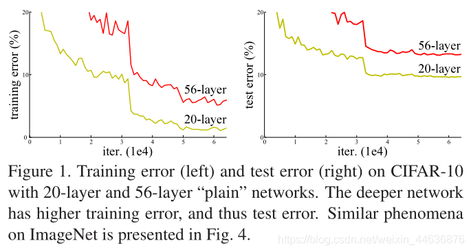
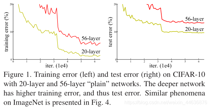
When deeper networks are able to start converging, a degradation problem has been exposed: with the network depth increasing, accuracy gets saturated (which might be unsurprising) and then degrades rapidly. Unexpectedly, such degradation is not caused by overfitting, and adding more layers to a suitably deep model leads to higher training error, as reported in [10, 41] and thoroughly verified by our experiments. Fig. 1 shows a typical example.
The degradation (of training accuracy) indicates that not all systems are similarly easy to optimize. Let us consider a shallower architecture and its deeper counterpart that adds more layers onto it. There exists a solution by construction to the deeper model: the added layers are identity mapping, and the other layers are copied from the learned shallower model. The existence of this constructed solution indicates that a deeper model should produce no higher training error than its shallower counterpart. But experiments show that our current solvers on hand are unable to find solutions that are comparably good or better than the constructed solution (or unable to do so in feasible time).
In this paper, we address the degradation problem by introducing a deep residual learning framework. Instead of hoping each few stacked layers directly fit a desired underlying mapping, we explicitly let these layers fit a residual mapping. Formally, denoting the desired underlying mapping as H(x), we let the stacked nonlinear layers fit another mapping of $F(x) := H(x)−x$. The original mapping is recast into $F(x)+x$. We hypothesize that it is easier to optimize the residual mapping than to optimize the original, unreferenced mapping. To the extreme, if an identity mapping were optimal, it would be easier to push the residual to zero than to fit an identity mapping by a stack of nonlinear layers.

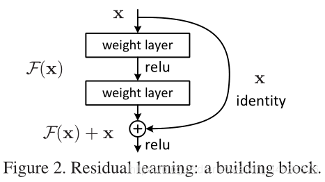
The formulation of $F(x)+x$ can be realized by feedforward neural networks with “shortcut connections” (Fig. 2). Shortcut connections [2, 33, 48] are those skipping one or more layers. In our case, the shortcut connections simply perform identity mapping, and their outputs are added to the outputs of the stacked layers (Fig. 2). Identity shortcut connections add neither extra parameter nor computational complexity. The entire network can still be trained end-to-end by SGD with backpropagation, and can be easily implemented using common libraries (e.g., Caffe [19]) without modifying the solvers.
We present comprehensive experiments on ImageNet [35] to show the degradation problem and evaluate our method. We show that: 1) Our extremely deep residual nets are easy to optimize, but the counterpart “plain” nets (that simply stack layers) exhibit higher training error when the depth increases; 2) Our deep residual nets can easily enjoy accuracy gains from greatly increased depth, producing results substantially better than previous networks.
Similar phenomena are also shown on the CIFAR-10 set [20], suggesting that the optimization difficulties and the effects of our method are not just akin to a particular dataset. We present successfully trained models on this dataset with over 100 layers, and explore models with over 1000 layers.
On the ImageNet classification dataset [35], we obtain excellent results by extremely deep residual nets. Our 152layer residual net is the deepest network ever presented on ImageNet, while still having lower complexity than VGG nets [40]. Our ensemble has 3.57% top-5 error on the ImageNet test set, and won the 1st place in the ILSVRC 2015 classification competition. The extremely deep representations also have excellent generalization performance on other recognition tasks, and lead us to further win the 1st places on: ImageNet detection, ImageNet localization,COCO detection, and COCO segmentation in ILSVRC & COCO 2015 competitions. This strong evidence shows that the residual learning principle is generic, and we expect that it is applicable in other vision and non-vision problems.

1.引言

深度卷积神经网络在图像分类上取得了很多的突破。深度网络通常通过端到端的方式将低、中、高级的特征和分类器集成在一起，并且特征的“级别”可以通过堆叠层的数量(深度)来丰富。最近的实验数据表明，网络深度至关重要，在ImageNet挑战上排名前列的网络通常深度都比较深，深度在16-30。深层网络对其他的重要模型也有很大的帮助。
网络的深度很重要，但同时也出现了另一个问题：深层网络的学习会像堆叠网络一样简单吗？大家熟知的网络越深可能会导致梯度消失或爆炸的问题，它从一开始就会阻碍收敛。但这个问题通过初始规范化和中间规范化解决了，十多层的网络能够收敛，并进行反向随机梯度下降传播。
当更深层的网络能够开始收敛时，退化的问题就暴露出来了：随着网络深度的增加，精度达到饱和（这可能并不奇怪），然后迅速下降。但这种退化并不是由过拟合引起的，而且在适当的深度模型中添加更多的层会导致更高的训练误差，对此我们进行了大量实验充分证实了这一点。图1示出了一个典型示例。

训练精度的下降表明并非所有的网络都容易优化。我们来思考一下一个浅层网络和它对应的深层网络。对于深层模型我们可以在浅层模型的基础上添加恒等映射层，即输出等于输入的层，构建出一个 deeper 网络。这两个网络（shallower 和 deeper）得到的结果应该是一模一样的，因为堆上去的层都是 identity mapping，其他层是从浅层模型复制的。这样可以得出一个结论：理论上，在训练集上，Deeper 不应该比 shallower 差，即越深的网络不会比浅层的网络效果差。但实验表明，我们无法在可行的时间内找到比构造解更好的解。
本文，我们通过引入一个深度残差模块框架来解决退化问题。假定某段神经网络的输入是 x，期望输出是 H(x)，即 H(x) 是期望的复杂潜在映射，但学习难度大；如果我们直接把输入 x 传到输出作为初始结果，那么此时我们需要学习的目标就是 $F(x)=H(x)-x$，于是 ResNet 相当于将学习目标改变了，不再是学习一个完整的输出，而是最优解 H(X) 和全等映射 x 的差值，即残差 $F(x) = H(x) - x$。 在极端情况下，如果一个恒等映射是最优的，那么将残差为零比用一堆非线性层来拟合恒等映射要容易得多。
$F(x)+x$的公式可以通过带shortcut connections的前馈神经网络实现(图2)。shortcut connections是跳过一层或多层的连接。在我们的例子中，shortcut connections只是执行标识映射，它们的输出被添加到堆叠层的输出中(图2)。标识shortcut connections既不增加额外的参数，也不增加计算复杂度。整个网络仍然可以通过SGD进行端到端的训练，并且可以使用框架轻松实现，而无需修改求解器。
我们在ImageNet上进行了全面的实验来表明退化问题并评估我们的方法。实验结果表明:1)极深残差网络很容易优化，但仅通过简单的堆叠的网络在深度增加时表现出更高的训练误差;2)残差网络大幅的提高了精度，产生的结果大大优于以前的网络。
在CIFAR-10数据集上也是差不多的结果，这表明我们的方法不仅仅适用于特定的数据集。我们成功的训练了超过100层的网络模型，并且探索了超过1000层的网络模型。
残差网络在ImageNet分类数据集上得到了很好的结果。我们的152层残差网络是ImageNet上迄今为止最深的网络，同时还比的VGG网复杂度低。我们网络在ImageNet测试集上top-5的误差为3.57%，在ILSVRC 2015分类竞赛中获得了第一名。极深的网络让其在其他识别任务上也有很好的泛化性能，在ILSVRC & COCO 2015年的比赛中，ImageNet 检测, ImageNet 定位, COCO 检测, COCO 分割都获得了第一名。这些都表明残差模块是通用的，我们也希望它能适用于其他视觉和非视觉问题。

2. Related Work

Residual Representations. In image recognition, VLAD [18] is a representation that encodes by the residual vectors with respect to a dictionary, and Fisher Vector [30] can be formulated as a probabilistic version [18] of VLAD. Both of them are powerful shallow representations for image retrieval and classification [4, 47]. For vector quantization, encoding residual vectors [17] is shown to be more effective than encoding original vectors.
In low-level vision and computer graphics, for solving Partial Differential Equations (PDEs), the widely used Multigrid method [3] reformulates the system as subproblems at multiple scales, where each subproblem is responsible for the residual solution between a coarser and a finer scale. An alternative to Multigrid is hierarchical basis preconditioning [44, 45], which relies on variables that represent residual vectors between two scales. It has been shown [3, 44, 45] that these solvers converge much faster than standard solvers that are unaware of the residual nature of the solutions. These methods suggest that a good reformulation or preconditioning can simplify the optimization.
Shortcut Connections. Practices and theories that lead to shortcut connections [2, 33, 48] have been studied for a long time. An early practice of training multi-layer perceptrons (MLPs) is to add a linear layer connected from the network input to the output [33, 48]. In [43, 24], a few intermediate layers are directly connected to auxiliary classifiers for addressing vanishing/exploding gradients. The papers of [38, 37, 31, 46] propose methods for centering layer responses, gradients, and propagated errors, implemented by shortcut connections. In [43], an “inception” layer is composed of a shortcut branch and a few deeper branches.
Concurrent with our work, “highway networks” [41, 42] present shortcut connections with gating functions [15]. These gates are data-dependent and have parameters, in contrast to our identity shortcuts that are parameter-free. When a gated shortcut is “closed” (approaching zero), the layers in highway networks represent non-residual functions. On the contrary, our formulation always learns residual functions; our identity shortcuts are never closed, and all information is always passed through, with additional residual functions to be learned. In addition, highway networks have not demonstrated accuracy gains with extremely increased depth (e.g., over 100 layers).

2.相关工作

残差表示：在图像识别中，VLAD是根据字典对残差向量进行编码的表示，Fisher向量可以表示为VLAD的概率版本。它们都是图像检索和分类的强大的浅层表示法。对于向量量化，编码残差向量比编码原始向量更有效。
在低级视觉和计算机图形学中，为了求解偏微分方程(PDEs)，广泛使用的多重网格方法将系统重新化为多尺度下的子问题，其中每个子问题负责在较粗尺度和较细尺度之间的残差解。另一个解法是分层基础预处理，是基于两个尺度的残差进行表示的。实验已经证明，使用残差求解比不使用的要快得多。这些研究表明，一个好的模型重构或者预处理手段是能简化优化过程的。
快捷连接：实践和理论引出了“快捷连接”这个想法，并且研究已久。在早期，训练多层感知器（mlp）是添加一个从网络输入连接到输出的线性层。[43，24]中提到，一些中间层直接连接到辅助分类器，用于处理消失/爆炸梯度。[38，37，31，46]的论文提出了用快捷连接解决对中层响应、梯度和传播误差的方法。在[43]中，“初始”层由一个快捷分支和几个更深的分支组成。
在我们的工作同期 ，“Highway Networks”高速公路网络提供了具有门控功能的快捷连接。这些门依赖于数据并且有参数，而我们的恒等连接是无参数的。当封闭的快捷方式“关闭”（接近零）时，公路网中的层就表示非残差函数。与此相反，我们的公式总是学习残差函数，恒等映射不会关闭，所以所有的信息都会通过，以借此来学习额外的残差函数。此外，高速网络并没有表现出深度极大增加（例如，超过100层）对精度提高的性能。

3. Deep Residual Learning

3.深度残差学习

3.1. Residual Learning

Let us consider $H(x)$ as an underlying mapping to be fit by a few stacked layers (not necessarily the entire net), with x denoting the inputs to the first of these layers. If one hypothesizes that multiple nonlinear layers can asymptotically approximate complicated functions , then it is equivalent to hypothesize that they can asymptotically approximate the residual functions, i.e., $H(x) −x$(assuming that the input and output are of the same dimensions). So rather than expect stacked layers to approximate $H(x)$, we explicitly let these layers approximate a residual function $F(x) := H(x) −x$. The original function thus becomes $F(x)+x$. Although both forms should be able to asymptotically approximate the desired functions (as hypothesized), the ease of learning might be different.
This reformulation is motivated by the counterintuitive phenomena about the degradation problem (Fig. 1, left). As we discussed in the introduction, if the added layers can be constructed as identity mappings, a deeper model should have training error no greater than its shallower counterpart. The degradation problem suggests that the solvers might have difficulties in approximating identity mappings by multiple nonlinear layers. With the residual learning reformulation, if identity mappings are optimal, the solvers may simply drive the weights of the multiple nonlinear layers toward zero to approach identity mappings.
In real cases, it is unlikely that identity mappings are optimal, but our reformulation may help to precondition the problem. If the optimal function is closer to an identity mapping than to a zero mapping, it should be easier for the solver to find the perturbations with reference to an identity mapping, than to learn the function as a new one. We show by experiments (Fig. 7) that the learned residual functions in general have small responses, suggesting that identity mappings provide reasonable preconditioning.

3.1残差学习

我们把$H(x)$看作是一个由多个堆叠层组成的底层映射，x表示这些层中第一个层的输入。如果假设多个非线性层可以渐近逼近复杂函数，那么就相当于假设它们可以渐近逼近残差函数，即$H(x)−x$（假设输入和输出具有相同的维数）。因此，我们不希望堆叠层近似H(x)，而是明确地让这些层近似于一个剩余函数$F(x)=H(x)−x$。因此，原始函数变成$F(x)+x$。尽管这两种形式都应该能够渐进地近似所需的函数（如假设的那样），但是学习的容易程度可能不同。

3.2. Identity Mapping by Shortcuts

We adopt residual learning to every few stacked layers. A building block is shown in Fig. 2. Formally, in this paper we consider a building block defined as:
$y=F(x,\left \{ W_{i} \right \})+x$ (1)
Here x and y are the input and output vectors of the layers considered. The function $F(x,\left \{ W_{i} \right \})$represents the residual mapping to be learned. For the example in Fig. 2 that has two layers, $F = W_{2\sigma }\left ( W_{1x} \right )$ in which σ denotes ReLU [29] and the biases are omitted for simplifying notations. The operation F + x is performed by a shortcut connection and element-wise addition. We adopt the second nonlinearity after the addition (i.e., σ(y), see Fig. 2).
The shortcut connections in Eqn.(1) introduce neither extra parameter nor computation complexity. This is not only attractive in practice but also important in our comparisons between plain and residual networks. We can fairly compare plain/residual networks that simultaneously have the same number of parameters, depth, width, and computational cost (except for the negligible element-wise addition). The dimensions of x and F must be equal in Eqn.(1). If this is not the case (e.g., when changing the input/output channels), we can perform a linear projection Ws by the shortcut connections to match the dimensions:
$y = F(x,\left \{ W_{i} \right \})+W_{s^{X}}$ (2)
We can also use a square matrix Ws in Eqn.(1). But we will show by experiments that the identity mapping is sufficient for addressing the degradation problem and is economical, and thus Ws is only used when matching dimensions.
The form of the residual function F is flexible. Experiments in this paper involve a function F that has two or three layers (Fig. 5), while more layers are possible. But if F has only a single layer, Eqn.(1) is similar to a linear layer:
$y=W_{1}x+x$, for which we have not observed advantages.
We also note that although the above notations are about fully-connected layers for simplicity, they are applicable to convolutional layers. The function $F(x,\left \{ W_{i} \right \})$can represent multiple convolutional layers. The element-wise addition is performed on two feature maps, channel by channel.

3.2通过快捷连接的恒等映射

我们对多层进行残差学习。图2示出了构建块。形式上，我们考虑将构建块定义为：
$y=F(x,\left \{ W_{i} \right \})+x$ (1)
其中x和y是所考虑层的输入和输出向量。函数$F(x,\left \{ W_{i} \right \})$表示要学习的剩余映射。对于图2中有两层的示例，$F = W_{2\sigma }\left ( W_{1^{X}} \right )$ ，其中σ表示ReLU,偏差被省略以简化符号。操作$F+x$是通过一个快捷连接和元素级加法来执行的。在加法操作后我们使用另一个非线性连接（即σ（y），见图2）。
（1）式中的快捷连接：既不引入额外参数，也不引入计算复杂度。这不仅是一个很有吸引力的做法，而且在我们比较plain网络和残差网络时也很重要。我们可以比较同时具有相同参数数量、深度、宽度和计算成本的plain网络和残差网络（除了可忽略的元素加法）。x和F的维度在等式（1）中必须相等。如果不相同（例如, 当改变了输入/输出的通道），我们可以通过shortcut连接执行一个线性映射Ws 来匹配两者的维度：
$y = F(x,\left \{ W_{i} \right \})+W_{s^{X}}$ (2)
我们也可以用一个方阵Ws来表示Eq1。但是实验证明恒等映射足以解决退化问题，并且是经济的，因此Ws只在匹配维度时使用。残差函数F的形式是灵活的。本文中的实验涉及一个具有两个或三个层的函数F（图5），但更多层也是可以的。但如果F只有一个层，则式（1）就类似于线性层：y=W1x+x，因此并不具有优势。我们还发现不仅是对于全连接层，对于卷积层也是同样适用的。函数$F(x,\left\{{Wi}\right\})$可以表示多个卷积层，在两个特征图的通道之间执行元素级的加法。

3.3. Network Architectures

We have tested various plain/residual nets, and have observed consistent phenomena. To provide instances for discussion, we describe two models for ImageNet as follows.

3.3网络结构

我们在多个plain网络和残差网络上进行了测试，并都观测到了一致的现象。接下来我们将在ImageNet上对两个模型进行讨论。
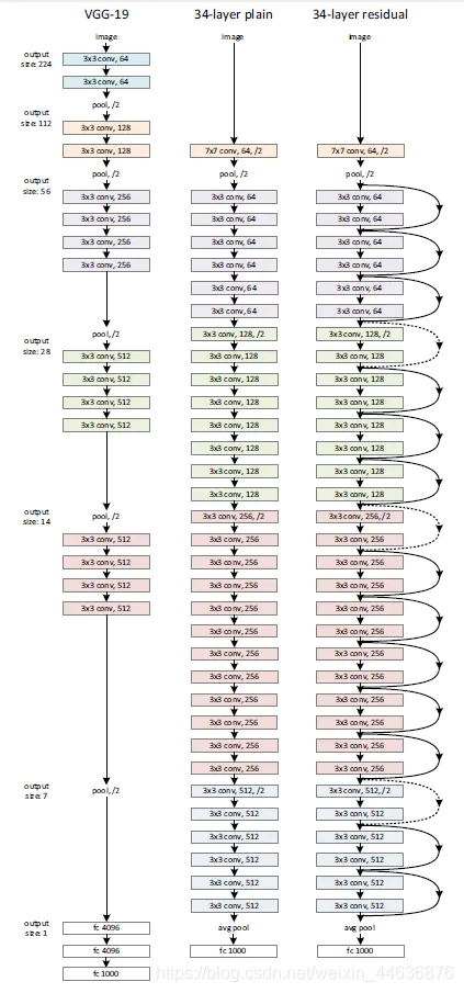
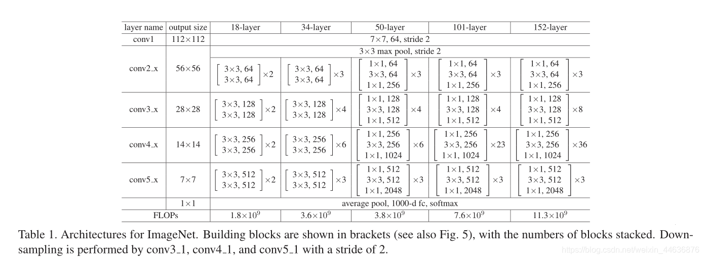
Plain Network. Our plain baselines (Fig. 3, middle) are mainly inspired by the philosophy of VGG nets [40] (Fig. 3, left). The convolutional layers mostly have 3×3 filters and follow two simple design rules: (i) for the same output feature map size, the layers have the same number of filters; and (ii) if the feature map size is halved, the number of filters is doubled so as to preserve the time complexity per layer. We perform downsampling directly by convolutional layers that have a stride of 2. The network ends with a global average pooling layer and a 1000-way fully-connected layer with softmax. The total number of weighted layers is 34 in Fig. 3 (middle).
It is worth noticing that our model has fewer filters and lower complexity than VGG nets [40] (Fig. 3, left). Our 34layer baseline has 3.6 billion FLOPs (multiply-adds), which is only 18% of VGG-19 (19.6 billion FLOPs).
plain网络：我们的plain网络结构（图3，中间）主要受VGG网络的启发（图3，左）。卷积层主要为3×3的滤波器，遵循两个简单的设计规则：（i）对于相同的输出特征映射大小，各层具有相同数量的滤波器；（ii）如果特征映射大小减半，则滤波器数量加倍，以保持每层的时间复杂度。我们直接通过2步的卷积层进行下采样。该网络以一个全局平均池层和一个1000路全连接层和softmax结束。图3（中间）中加权层的总数为34。
值得注意的是，我们的模型比VGG网络滤波器更少，复杂性更低。（图3，左图）。我们34层的结构含有36亿个FLOPs（乘-加），而这仅仅只有VGG-19 （196亿个FLOPs）的18%。

Residual Network. Based on the above plain network, we insert shortcut connections (Fig. 3, right) which turn the network into its counterpart residual version. The identity shortcuts (Eqn.(1)) can be directly used when the input and output are of the same dimensions (solid line shortcuts in Fig. 3). When the dimensions increase (dotted line shortcuts
in Fig. 3), we consider two options: (A) The shortcut still performs identity mapping, with extra zero entries padded for increasing dimensions. This option introduces no extra parameter; (B) The projection shortcut in Eqn.(2) is used to match dimensions (done by 1×1 convolutions). For both
options, when the shortcuts go across feature maps of two sizes, they are performed with a stride of 2.
残差网络
基于上述plain网络，我们插入快捷连接（图3，右图），将网络转换为对应的残差版本。当输入和输出具有相同的尺寸（图3中的实线快捷方式）时，可以直接使用快捷连接（Eqn.（1））。当维度增加时（图3中的虚线快捷方式），我们考虑两个方法：
（A）快捷方式仍然执行恒等映射，并为增加维度填零。此方法不引入额外参数；
（B）利用公式（2）中的映射快捷方式来使维度 保持一致（通过1×1卷积完成）。
对于这两个方法，当shortcut跨越两种尺寸的特征图时，均使用stride为2的卷积。

3.4. Implementation

Our implementation for ImageNet follows the practice in [21, 40]. The image is resized with its shorter side randomly sampled in [256,480] for scale augmentation [40].A 224×224 crop is randomly sampled from an image or its horizontal flip, with the per-pixel mean subtracted [21]. The standard color augmentation in [21] is used. We adopt batch normalization (BN) [16] right after each convolution and before activation, following [16]. We initialize the weights as in [12] and train all plain/residual nets from scratch. We use SGD with a mini-batch size of 256. The learning rate starts from 0.1 and is divided by 10 when the error plateaus,and the models are trained for up to 60×104iterations. We use a weight decay of 0.0001 and a momentum of 0.9. We do not use dropout [13], following the practice in [16].
In testing, for comparison studies we adopt the standard 10-crop testing [21]. For best results, we adopt the fully-convolutional form as in [40, 12], and average the scores at multiple scales (images are resized such that the shorter side is in {224,256,384,480,640}).

3.4应用

我们对ImageNet的实现遵循了Krizhevsky2012ImageNet
和Simonyan2014Very中的实践。调整图像的大小使它的短边长度随机的从[256,480] 中采样来增大图像的尺寸。从图像或其水平翻转中随机裁取224×224大小的图像，并减去每个像素的平均值。图像使用标准颜色增强。在每次卷积后和激活前采用批处理标准化（BN）。按照K. He2015中的方法初始化权重，并从头开始训练所有的plain网络和残差网络。使用SGD，最小批量为256。学习率从0.1开始，每当误差趋于平稳时除以10，模型训练迭代$60\ast 10^4$次。使用0.0001的重量衰减和0.9的动量，并且不使用dropout。在测试中，为了进行比较，我们采取标准的10-crop测试。为了获得最佳结果，我们采用Krizhevsky2012ImageNet和K. He2015中的全卷积形式，并在多个尺度上对分数进行平均（调整图像大小，使短边位于{224，256，384，480，640}）。

4. Experiments

4.实验

4.1. ImageNet Classification

We evaluate our method on the ImageNet 2012 classification dataset [35] that consists of 1000 classes. The models are trained on the 1.28 million training images, and evaluated on the 50k validation images. We also obtain a final result on the 100k test images, reported by the test server. We evaluate both top-1 and top-5 error rates.

4.1. ImageNet 分类

我们在包含1000个类的ImageNet 2012分类数据集上评估我们的方法。训练集有128万张图像，测试集有5万张图像。最终在10万张图像上进行测试，并对top-1和top-5 的错误率进行评估。
Plain Networks. We first evaluate 18-layer and 34-layer plain nets. The 34-layer plain net is in Fig. 3 (middle). The 18-layer plain net is of a similar form. See Table 1 for detailed architectures.

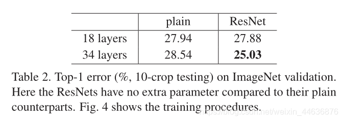
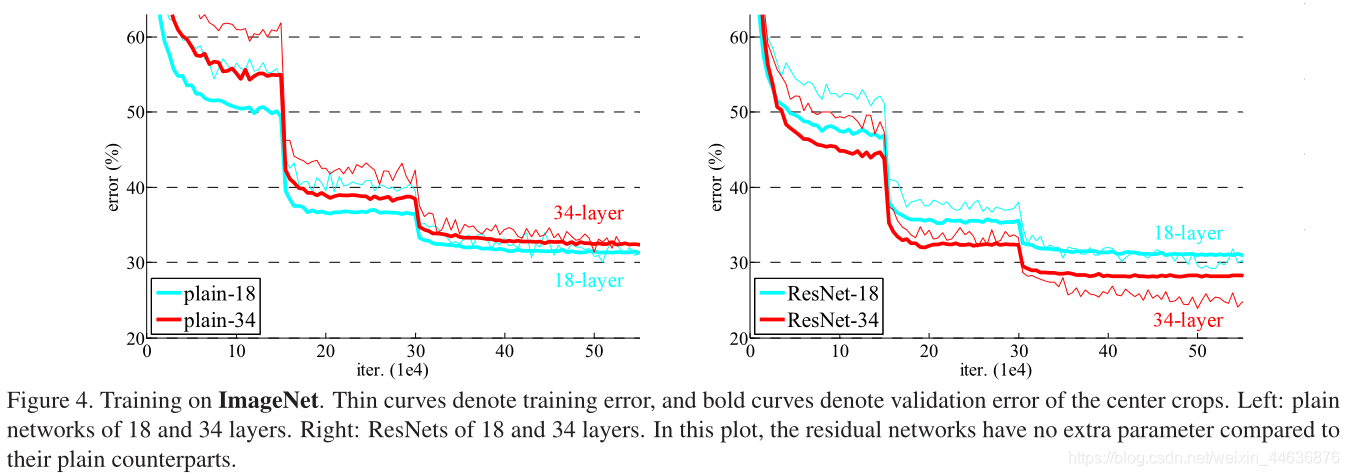
The results in Table 2 show that the deeper 34-layer plain net has higher validation error than the shallower 18-layer plain net. To reveal the reasons, in Fig. 4 (left) we compare their training/validation errors during the training procedure. We have observed the degradation problem - the 34-layer plain net has higher training error throughout the whole training procedure, even though the solution space of the 18-layer plain network is a subspace of that of the 34-layer one.

We argue that this optimization difficulty is unlikely to be caused by vanishing gradients. These plain networks are trained with BN [16], which ensures forward propagated signals to have non-zero variances. We also verify that the backward propagated gradients exhibit healthy norms with BN. So neither forward nor backward signals vanish. In fact, the 34-layer plain net is still able to achieve competitive accuracy (Table 3), suggesting that the solver works to some extent. We conjecture that the deep plain nets may have exponentially low convergence rates, which impact the reducing of the training error . The reason for such optimization difficulties will be studied in the future.
首先评估18层和34层plain网络。图3（中）为34层plain网络。18层plain网络形式相似。具体架构见表1。
Table 2中展示的结果表明了34层的网络比18层的网络具有更高的验证错误率。为了揭示产生这种现象的原因，在Fig.4(左)中我们比较了整个训练过程中的训练及验证错误率。从结果中我们观测到了明显的退化问题——在整个训练过程中34 层的网络具有更高的训练错误率，即使18层网络的解空间为34层解空间的一个子空间。
我们认为这种优化困难不太可能是由梯度消失引起的。训练plain网络时使用BN，这能保证前向传递的信号是具有非零方差的。我们还验证了反向传播的梯度与BN具有良好的规范性。所以前馈和反向传播的信号都不会消失。实际上，34层plain网络仍然能够达到竞争的精度（表3），这表明求解器在一定程度上起作用。我们推测深层的plain网络的收敛率是指数衰减的，这可能会影响训练误差的降低。这种困难优化我们将在以后进行研究。
Residual Networks. Next we evaluate 18-layer and 34layer residual nets (ResNets). The baseline architectures are the same as the above plain nets, expect that a shortcut connection is added to each pair of 3×3 filters as in Fig. 3 (right). In the first comparison (Table 2 and Fig. 4 right), we use identity mapping for all shortcuts and zero-padding for increasing dimensions (option A). So they have no extra parameter compared to the plain counterparts.
We have three major observations from Table 2 and Fig. 4. First, the situation is reversed with residual learning – the 34-layer ResNet is better than the 18-layer ResNet (by 2.8%). More importantly, the 34-layer ResNet exhibits considerably lower training error and is generalizable to the validation data. This indicates that the degradation problem is well addressed in this setting and we manage to obtain accuracy gains from increased depth.
Second, compared to its plain counterpart, the 34-layer ResNet reduces the top-1 error by 3.5% (Table 2), resulting from the successfully reduced training error (Fig. 4 right vs. left). This comparison verifies the effectiveness of residual learning on extremely deep systems.
Last, we also note that the 18-layer plain/residual nets are comparably accurate (Table 2), but the 18-layer ResNet converges faster (Fig. 4 right vs. left). When the net is “not overly deep” (18 layers here), the current SGD solver is still able to find good solutions to the plain net. In this case, the ResNet eases the optimization by providing faster convergence at the early stage.
残差网络。接下来我们评估18层和34层残差网络（ResNets）。ResNets架构与plain网络相同，只是在每对3×3滤波器上增加了一个快捷连接，如图3（右图）所示。在第一个比较中（表2和图4右图），我们对所有快捷方式使用恒等映射，增加的维度使用零填充（选项A）。因此，与普通的网络相比，没有增加额外的参数。表2和图4体现了我们三个主要的观察结果。首先，通过残差学习扭转了这种情况——34层ResNet比18层ResNet好（2.8%）。更重要的是，34层ResNet显示出相当低的训练误差，并且可以推广到验证数据中。这表明，在这种情况下，退化问题得到了很好的解决，我们设法从增加深度中获得精度增益。
第二，与普通的34层相比ResNet top-1错误减少了3.5%（表2），因为训练误差减少了 （图4右与左）。这种比较验证了残差学习在极深系统上的有效性。
最后，我们还注意到18层plain网络和残差网络准确率差不多（表2），但18层ResNet收敛更快（图4右对左）。当网络“不太深”（这里是18层）时，现有的SGD能够很好的对plain网络进行求解，而ResNet能够使优化得到更快的收敛。



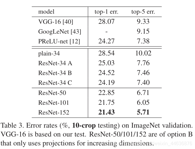
Identity vs. Projection Shortcuts. We have shown that parameter-free, identity shortcuts help with training. Next we investigate projection shortcuts (Eqn.(2)). In Table 3 we compare three options: (A) zero-padding shortcuts are used for increasing dimensions, and all shortcuts are parameterfree (the same as Table 2 and Fig. 4 right); (B) projection shortcuts are used for increasing dimensions, and other shortcuts are identity; and © all shortcuts are projections.

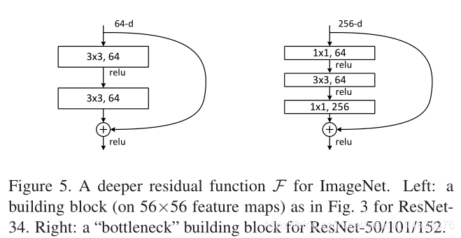
Table 3 shows that all three options are considerably better than the plain counterpart. B is slightly better than A. We argue that this is because the zero-padded dimensions in A indeed have no residual learning. C is marginally better than B, and we attribute this to the extra parameters introduced by many (thirteen) projection shortcuts. But the small differences among A/B/C indicate that projection shortcuts are not essential for addressing the degradation problem. So we do not use option C in the rest of this paper, to reduce memory/time complexity and model sizes. Identity shortcuts are particularly important for not increasing the complexity of the bottleneck architectures that are introduced below.
恒等vs映射快捷连接
已经验证了无参数的恒等快捷连接是有助于训练的。接下来我们研究映射快捷连接方式（Eqn.（2））。在表3中，我们比较了三个选项：
（A）零填充快捷键用于增加维度，并且所有快捷链接都是无参数的（与表2和图4右相同）；
（B）增加的维度使用映射快捷连接，其他的使用恒等快捷连接；
（C）都是用映射快捷连接。
表3显示，这三种方案都比plain模型好得多。B略好于A，我们认为这是因为A中的0填充并没有进行残差学习。C略优于B，我们将其归因于多个映射快捷链接引入了额外参数。但是A/B/C之间的细微差别表明，映射快捷方式对于解决退化问题不是必需的。因此，在本文的其余部分中，我们不使用选项C来降低内存/时间复杂性和模型大小。恒等快捷连接对于不增加下面介绍的瓶颈体系结构的复杂性特别重要。
Deeper Bottleneck Architectures. Next we describe our deeper nets for ImageNet. Because of concerns on the training time that we can afford, we modify the building block as a bottleneck design . For each residual function F, we use a stack of 3 layers instead of 2 (Fig. 5). The three layers are 1×1, 3×3, and 1×1 convolutions, where the 1×1 layers are responsible for reducing and then increasing (restoring) dimensions, leaving the 3×3 layer a bottleneck with smaller input/output dimensions. Fig. 5 shows an example, where both designs have similar time complexity.
The parameter-free identity shortcuts are particularly important for the bottleneck architectures. If the identity shortcut in Fig. 5 (right) is replaced with projection, one can show that the time complexity and model size are doubled, as the shortcut is connected to the two high-dimensional ends. So identity shortcuts lead to more efficient models for the bottleneck designs.
50-layer ResNet: We replace each 2-layer block in the 34-layer net with this 3-layer bottleneck block, resulting in a 50-layer ResNet (Table 1). We use option B for increasing dimensions. This model has 3.8 billion FLOPs.
101-layer and 152-layer ResNets: We construct 101layer and 152-layer ResNets by using more 3-layer blocks (Table 1). Remarkably, although the depth is significantly increased, the 152-layer ResNet (11.3 billion FLOPs) still has lower complexity than VGG-16/19 nets (15.3/19.6 billion FLOPs).
The 50/101/152-layer ResNets are more accurate than the 34-layer ones by considerable margins (Table 3 and 4). We do not observe the degradation problem and thus enjoy significant accuracy gains from considerably increased depth. The benefits of depth are witnessed for all evaluation metrics (Table 3 and 4).
深层瓶颈结构
接下来，我们将描述ImageNet的深层网络。出于对训练时间的考虑，我们将构建块修改为瓶颈设计。对于每个剩余函数F，我们使用3层而不是2层的堆栈（图5）。这三个层分别是1×1、3×3和1×1卷积，其中1×1层负责减少然后增加（恢复）维度，使3×3层成为输入/输出维数较小的瓶颈。图5示出了两个设计具有相似的时间复杂度。
无参数恒等快捷链接对于瓶颈体系结构尤为重要。如果将图5（右）中的恒等快捷连接替换为映射快捷连接，模型的时间复杂度和时间复杂度都会加倍，因为快捷连接到了两个高维端。所以恒等连接对于瓶颈设计是更加有效的。
50层ResNet：我们将34层网络中2层的模块替换成3层的瓶颈模块，整个模型也就变成了50层的ResNet (Table 1)。对于增加的维度我们使用选项B来处理。整个模型含有38亿个FLOPs。
101层和152层resnet：我们使用更多的3层块构建101层和152层ResNet（表1）。值得注意的是，尽管深度显著增加，但152层ResNet（113亿个FLOPs）仍然比VGG-16/19网络（153/196亿个FLOPs）的复杂度低。
50/101/152层ResNet比34层ResNet精度高出相当多（表3和表4）。并且我们没有观察到退化问题，因此网络得加深可以对精度提升较好的效果。深度的好处在所有评估指标中都有体现（表3和表4）。
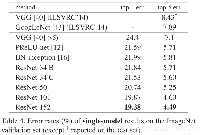
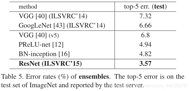
Comparisons with State-of-the-art Methods. In Table 4 we compare with the previous best single-model results. Our baseline 34-layer ResNets have achieved very competitive accuracy. Our 152-layer ResNet has a single-model top-5 validation error of 4.49%. This single-model result outperforms all previous ensemble results (Table 5). We combine six models of different depth to form an ensemble (only with two 152-layer ones at the time of submitting). This leads to 3.57% top-5 error on the test set (Table 5). This entry won the 1st place in ILSVRC 2015.
与最先进方法的比较。在表4中，我们将与之前的最佳单模型结果进行比较。我们的34层ResNets 已经达到了非常有竞争力的准确性。152层ResNet TOP-5验证误差仅为4.49%。这个结果优于所有先前的集合结果（表5）。我们将6个不同深度的ResNets合成一个组合模型(在提交结果时只用到2个152层的模型)。这在测试集上的top-5错误率仅为3.57% (表5)，这一项在ILSVRC 2015 上获得了第一名的成绩。

4.2. CIFAR-10 and Analysis

We conducted more studies on the CIFAR-10 dataset [20], which consists of 50k training images and 10k testing images in 10 classes. We present experiments trained on the training set and evaluated on the test set. Our focus is on the behaviors of extremely deep networks, but not on pushing the state-of-the-art results, so we intentionally use simple architectures as follows.
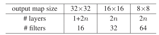
The plain/residual architectures follow the form in Fig. 3 (middle/right). The network inputs are 32×32 images, with the per-pixel mean subtracted. The first layer is 3×3 convolutions. Then we use a stack of 6n layers with 3×3 convolutions on the feature maps of sizes {32,16,8} respectively, with 2n layers for each feature map size. The numbers of filters are {16,32,64} respectively. The subsampling is performed by convolutions with a stride of 2. The network ends with a global average pooling, a 10-way fully-connected layer, and softmax. There are totally 6n+2 stacked weighted layers. The following table summarizes the architecture:

When shortcut connections are used, they are connected to the pairs of 3×3 layers (totally 3n shortcuts). On this dataset we use identity shortcuts in all cases (i.e., option A),so our residual models have exactly the same depth, width, and number of parameters as the plain counterparts.

We use a weight decay of 0.0001 and momentum of 0.9, and adopt the weight initialization in [12] and BN [16] but with no dropout. These models are trained with a minibatch size of 128 on two GPUs. We start with a learning rate of 0.1, divide it by 10 at 32k and 48k iterations, and terminate training at 64k iterations, which is determined on a 45k/5k train/val split. We follow the simple data augmentation in [24] for training: 4 pixels are padded on each side, and a 32×32 crop is randomly sampled from the padded image or its horizontal flip. For testing, we only evaluate the single view of the original 32×32 image.
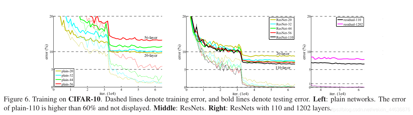
We compare n = {3,5,7,9}, leading to 20, 32, 44, and 56-layer networks. Fig. 6 (left) shows the behaviors of the plain nets. The deep plain nets suffer from increased depth, and exhibit higher training error when going deeper. This phenomenon is similar to that on ImageNet (Fig. 4, left) and on MNIST (see [41]), suggesting that such an optimization difficulty is a fundamental problem.
Fig. 6 (middle) shows the behaviors of ResNets. Also similar to the ImageNet cases (Fig. 4, right), our ResNets manage to overcome the optimization difficulty and demonstrate accuracy gains when the depth increases.
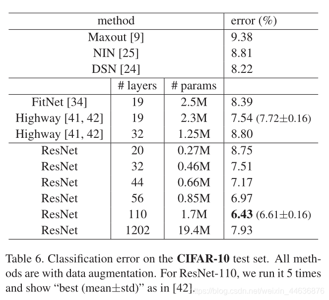
We further explore n = 18 that leads to a 110-layer ResNet. In this case, we find that the initial learning rate of 0.1 is slightly too large to start converging . So we use 0.01 to warm up the training until the training error is below 80% (about 400 iterations), and then go back to 0.1 and continue training. The rest of the learning schedule is as done previously. This 110-layer network converges well (Fig. 6, middle). It has fewer parameters than other deep and thin networks such as FitNet [34] and Highway [41] (Table 6), yet is among the state-of-the-art results (6.43%, Table 6).

4.2. CIFAR-10分析

我们对CIFAR-10数据集进行了更多的研究，该数据集包括10个类，训练集5万张图像，测试集1万张图像。我们在训练集上训练，并在测试集上进行了评估。我们关注的是验证极深模型的效果，而不是追求最好的结果，因此我们只使用简单的框架如下。Plain网络和残差网络的框架如 Fig.3(中/右)所示。网络的输入是$32*32$的减掉像素均值的图像。第一层是$3*3$的卷积层。然后我们使用6n个$3*3$的卷积层的堆叠，卷积层对应的特征图有三种：{32,16,8}，每一种卷积层的数量为2n 个，对应的滤波器数量分别为{16,32,64}。使用strde为2的卷积层进行下采样。在网络的最后是一个全局的平均pooling层和一个10类的包含softmax的全连接层。一共有6n+2个堆叠的加权层。具体的结构见下表：

当使用快捷方式连接$3\ast 3$卷积层对（共3n个快捷连接）。在这个数据集中，我们在所有情况下都使用恒等快捷链接方式（即选项A），因此，我们的残差模型具有与plain模型完全相同的深度、宽度和参数数量。采用了K. He2015中的权值初始化以及BN，但是不使用Dropout，mini-batch的大小为128，模型在2块GPU 上进行训练。我们从0.1的学习率开始，在第32k和48k次迭代时除以10，总训练次数为64k，这是根据45k/5k训练集/val测试确定的。我们使用简单的数据扩充方法进行训练：每边填充4个像素，从填充图像或其水平翻转中随机裁剪$32*32$大小图像。为了测试，我们只评估原始$32*32$图像的单个视图。
我们比较了n={3,5,7,9}，即20、32、44和56层网络。图6（左）显示了plain网络的结果。网络越深plain网络的训练误差越大。这种现象类似于ImageNet（图4，左图）和MNIST，这表明这种优化困难是一个基本问题。图6（中间）显示了ResNet的结果。同样类似于ImageNet的例子（图4，右图），ResNet设法克服了优化的困难，并且证明了随着深度的增加，精度得到了提高。

我们进一步研究n=18的情况，此时ResNet有110层。在这种情况下，我们发现初始学习率0.1无法开始收敛。所以我们用0.01预热训练直到训练误差小于80%（大约400次迭代），然后回到0.1继续训练。剩余的学习和之前的一样。这个110层网络收敛性很好（图6，中间）。它与其他的深层窄模型，如FitNet和 Highway (表6)相比，具有更少的参数，然而却达到了最好的结果 (6.43%, 表 6)。

Analysis of Layer Responses. Fig. 7 shows the standard deviations (std) of the layer responses. The responses are the outputs of each 3×3 layer, after BN and before other nonlinearity (ReLU/addition). For ResNets, this analysis reveals the response strength of the residual functions. Fig. 7 shows that ResNets have generally smaller responses than their plain counterparts. These results support our basic motivation (Sec.3.1) that the residual functions might be generally closer to zero than the non-residual functions. We also notice that the deeper ResNet has smaller magnitudes of responses, as evidenced by the comparisons among ResNet-20, 56, and 110 in Fig. 7. When there are more layers, an individual layer of ResNets tends to modify the signal less.

层响应分析
图7显示了层响应的标准偏差（std）。响应是每个3×3 BN之后和其他非线性函数（ReLU/addition）之前的输出。对于ResNets，这个分析结果也揭示了残差函数的响应强度。图7示出ResNet通常比它们的plain网络具有更小的响应。这些结果验证了我们的基本动机（第3.1节），即残差函数可能比非残差函数更接近于0。我们还注意到更深的ResNet具有较小的响应量，如图7中ResNet-20、56和110。当有更多层时，单个ResNet层倾向于减少信号的修改。

Exploring Over 1000 layers. We explore an aggressively deep model of over 1000 layers. We set n = 200 that leads to a 1202-layer network, which is trained as described above. Our method shows no optimization difficulty, and this 103-layer network is able to achieve training error <0.1% (Fig. 6, right). Its test error is still fairly good (7.93%, Table 6).
But there are still open problems on such aggressively deep models. The testing result of this 1202-layer network is worse than that of our 110-layer network, although both have similar training error. We argue that this is because of overfitting. The 1202-layer network may be unnecessarily large (19.4M) for this small dataset. Strong regularization such as maxout [9] or dropout [13] is applied to obtain the best results ([9, 25, 24, 34]) on this dataset. In this paper, we use no maxout/dropout and just simply impose regularization via deep and thin architectures by design, without distracting from the focus on the difficulties of optimization. But combining with stronger regularization may improve results, which we will study in the future.


探索超过1000层网络
我们探索了一个超过1000层的深度模型。我们将设n=200，有1202层网络，该网络按上述方式训练。对于这个$10^{3}$层网络我们同样能够优化，并且能够达到训练误差<0.1%（图6，右图）。其测试误差仍相当好（7.93%，表6）。
但这种极深的模型，仍然存在一些开放性的问题。该1202层网络的测试结果比我们的110层网络的测试结果要差，虽然都有训练误差都差不多。我们认为这是因为过拟合。1202层网络对于这个小数据集来说可能太大了（19.4M）。在该数据集上使用强正则化（如maxout或dropout）才获得了最佳结果。在本文中，我们没有使用maxout或dropout，只是通过设计简单地通过深层窄模型实施正则化，而不分散对优化困难的关注。我们将在以后研究结合更强的正则化对结果的提高作用。

4.3. Object Detection on PASCAL and MS COCO

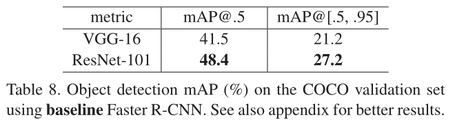
Our method has good generalization performance on other recognition tasks. Table 7 and 8 show the object detection baseline results on PASCAL VOC 2007 and 2012 [5] and COCO [26]. We adopt Faster R-CNN [32] as the detection method. Here we are interested in the improvements of replacing VGG-16 [40] with ResNet-101. The detection implementation (see appendix) of using both models is the same, so the gains can only be attributed to better networks. Most remarkably, on the challenging COCO dataset we obtain a 6.0% increase in COCO’s standard metric (mAP@[.5, .95]), which is a 28% relative improvement. This gain is solely due to the learned representations.
Based on deep residual nets, we won the 1st places in several tracks in ILSVRC & COCO 2015 competitions: ImageNet detection, ImageNet localization, COCO detection, and COCO segmentation. The details are in the appendix.

4.3 PASCAL 、MS COCO上的目标检测

我们的方法在其他识别任务上具有良好的泛化性能。表7和表8显示了PASCAL VOC 2007、2012和COCO的目标检测结果。我们采用Fast R-CNN作为检测方法。这里我们比较关注用ResNet-101代替VGG-16对结果的提升。对这两种模型的检测实现是一样的，因此有提升只能是由于这个网络更好。最值得注意的是，在具有挑战性的COCO数据集上，COCO的标准度量值（mAP@[.5，.95]）增加了6.0%，相对提高了28%。这种增益完全是由于学习的表现。基于深度残差网，我们在ILSVRC&COCO 2015竞赛中获得了多个赛道的第一名：ImageNet检测、ImageNet定位、COCO检测和COCO分割。详情见附录。

5.参考文献

References