手把手计算Dubins曲线

文章直接搬过来，原文：https://gieseanw.wordpress.com/2012/10/21/a-comprehensive-step-by-step-tutorial-to-computing-dubins-paths/

原文图不全，可以看PDF:https://gieseanw.files.wordpress.com/2012/10/dubins.pdf

大学教程http://planning.cs.uiuc.edu/node821.html

Imagine you have a point, a single little dot on a piece of paper. What’s the quickest way to go from that point to another point on the piece of paper? You (the reader) sigh and answer ”A straight line” because it’s completely obvious; even first graders know that. Now let’s imagine you have an open parking lot, with a human standing in it. What’s the quickest way for the human to get from one side of the parking lot to the other? The answer is again obvious to you, so you get a little annoyed and half-shout ”A straight-line again, duh!”. Okay, okay, enough toss-up questions. Now what if I gave you a car in the parking lot and asked you what was the quickest way for that car to get into a parking spot? Hmm, a little harder now.

You can’t say a straight line because what if the car isn’t facing directly towards the parking space? Cars don’t just slide horizontally and then turn in place, so planning for them seems to be a lot more difficult than for a human. But! We can make planning for a car just about as easy as for a human if we consider the car to be a special type of car we’ll call aDubin’s Car. Interested in knowing how? Then read on!

In robotics, we would consider our human from the example above to be a type of holonomic agent. Don’t let this terminology scare you; I’ll explain it all. A holonomic agent can simply be considered an agent who we have full control over. That is, if we treat the human as a point in the x-y plane, we are able to go from any coordinate to any other coordinate always. Humans can turn on a dime, walk straight forward, side-step, walk backwards, etc. They really have full control over their coordinates.
A car however, is not holonomic because we don’t have full control over it at all times. Therefore we call a car a type of nonholonomic agent.
Cars can only turn about some minimal radius circle, therefore they can’t move straight towards a point just barely to their left or right. As you can imagine, planning paths for nonholonomic agents is much more difficult than for holonomic ones.

Let’s simplify our model of our car. How about this: it can only move forwards — never backwards, and it’s always moving at a unit velocity so we don’t have to worry about braking or accelerating. What I just described is known as a Dubin’s car, and planning shortest paths for it is a well studied problem in robotics and control theory. What makes the Dubin’s car attractive is that its shortest paths can be solved exactly using relatively simple geometry, whereas planning for many other dynamical systems requires some pretty high level and complicated matrix operations.

The Dubin’s Car only moves forward, never backwards, even if reversal leads to a shorter path.

The Dubin’s Car was introduced into the literature by Lester Dubins, a famous mathematician and statistician, in a paper published in 1957. The cars essentially have only 3 controls: “turn left at maximum”, “turn right at maximum”, and “go straight”. All the paths traced out by the Dubin’s car are combinations of these three controls. Let’s name the controls: “turn left at maximum” will be L, “turn right at maximum” will be R, and “go straight” will be S. We can make things even more general: left and right turns both describe curves, so lets group them under a single category that we’ll call C (”curve”). Lester Dubins proved in his paper that there are only 6 combinations of these controls that describe ALL the shortest paths, and they are:RSR, LSL, RSL, LSR, RLR, and LRL. Or using our more general terminology, there’s only two classes:CSC andCCC.

Despite being relatively well studied, with all sorts of geometric proofs out there and qualitative statements about what the shortest paths look like, I could not find one single source on the internet that described in depth how to actually compute these shortest paths! So what that we know the car can try to turn left for some amount of time, then move straight, and then move right — I want to know exactly how much I need to turn, and how long I need to turn for. And if you’re like me in the least, you tend to forget some geometry that you learned in high school, so doing these computations isn’t as “trivial” for you like all the other online sources make it out to be.

If you’re looking for the actual computations needed to compute these shortest paths, then you’ve come to the right place. The following will be my longest article to-date, and is basically a how-to guide on computing the geometry required for the Dubin’s shortest paths.

Overview

This blog post was originally written in $\LaTeX$ and then transcribed here to WordPress. If you’d like a more portable, possibly easier to read version, then download the PDF version here (You may also cite this pdf if you’re writing a bibliography).

Let’s first talk about the dynamics of our system, and then describe in general terms what the shortest paths look like. Afterwards, I’ll delve into the actual calculations. Car-like robots all have one thing in common — they have a minimum turning radius. Think of this minimum turning radius as a circle next to the car that, try as it might, the robot can only go around the circle’s circumference if it turns as hard as it can. The radius of this circle, $r_{min}$ is the car’s minimum turning radius. This radius is determined by the physics of the car $\gets$ the maximum angle the tires can deviate from “forward”, and the car’s wheelbase, or the length from the front axle to rear axle.Marco Monster has a really good descriptive article that talks about these car dynamics.

Car Dynamics

I already mentioned that the Dubin’s car could only move forward at a unit velocity, and by “forward” I mean it can’t change gears into reverse. Let’s describe the vehicle dynamics more formally. A Car’s configuration can be describe by the triplet $\langle x, y, \theta \rangle$ . Define the car’s velocity (actually speed, because it will be a scalar quantity) as $v$ . When a car is moving at velocity $v$ about a circle of radius $r_{turn}$ , it will have angular velocity

$\omega = \frac{v}{r_{turn}}$

Now let’s define how our system evolves over time. If you know even just the basics of differential equations, this will be cake for you. If not, I’ll explain. When we want to describe how our system evolves over time, we use notation like $\dot{x}$ to talk about how our x coordinate changes over time.

In basic vector math, if our car is at position $A = \left(x_1, y_1\right)$ with $\theta = \theta_1$ , and we move straight forward for a single timestep, then our new configuration is $B = \left(x_1+vcos\left(\theta_1\right), y_1+vsin\left(\theta_1\right), \theta_1\right)$ Note how our $x$ coordinate changes as a function of $cos\left(\theta\right)$ . Therefore, we’d say that $\dot{x} = cos\left(\theta\right)$ . A full system description would read like this:

$\dot{x} = cos\left(\theta\right)$

$\dot{y} = sin\left(\theta\right)$

$\dot{\theta} = \omega = \frac{v}{r_{turn}}$

I’d like to point out that this equation is linear in that the car’s new position is changing to be some straight line away from the previous one. In reality, this is not the case; cars are nonlinear systems. Therefore, the dynamics I described above are merely an approximation of the true system dynamics. Linear systems are much easier to handle, and if we do things right, they can approximate the true dynamics so well that you’d never be able to tell the difference. The dynamics equations translate nicely into update equations. These update equations describe what actually happens each time you want to update the car’s configuration. That is, if you’re stepping through your simulator, at each timestep you’d want to update the car. As the Dubin’s car only has unit velocity, we’ll replace all instances of $v$ with $1$ .

$x_{new} = x_{prev} + \delta*cos\left(\theta\right)$

$y_{new} = y_{prev} + \delta*sin\left(\theta\right)$

$\theta_{new} = \theta_{prev} + \frac{\delta}{r_{turn}}$

Note that I actually replaced instances of $v$ with the symbol $\delta$ . What’s with that? Well, remember when I said that our dynamics are a linear approximation of a nonlinear system? Every time we update, we are moving the car along a line. If we only move a very short amount on this line, then we approximate turns more finely. Think of it this way: You are trying to draw a circle using a series of evenly-spaced points. If you only use 3 points, you get a triangle. If you use 4 you get a square, and 8 you get an octagon. As you add more and more points you get something that more closely resembles the circle. This is the same concept. $\delta$ essentially tells us the amount of spacing between our points. If it is really small, then the points are close together and we get overall motion that looks closer to reality.

High-level Description of Dubin’s curves

In this section I’ll briefly go over what each of the 6 trajectories (RSR, LSR, RSL, LSR, RLR, LRL) looks like. (Disclaimer:I do not claim to be an artist, and as such the figures you see that I drew in the following sections are NOT to scale; they merely serve to illustrate all the geometry being discussed.)

CSC Trajectories

The CSC trajectories include RSR, LSR,RSL, andLSR — a turn followed by a straight line followed by another turn (Shown in Figure 1).

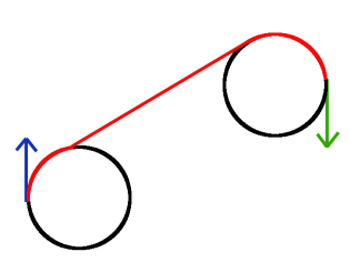
Figure 1. A RSR Trajectory

Pick a position and orientation for your start and goal configurations. Draw your start and goal configurations as points in the plane with arrows extending out in the direction the car is facing. Next, draw circles to the left and right of the car with radius $r_{min}$ . The circles should be tangent at the location of the car. Draw tangent lines from the circles at the starting configuration to the circles at the goal configuration. In the next section I’ll discuss how to compute this, but for now just draw them.

For each pair of circles (RR), (LL), (RL), (LR), there should be four possible tangent lines, but note that there is only one valid line for each pair (Shown in Figure 2. That is, for the RR circles, only one line extending from the agent’s circle meets the goal’s circle such that everything is going in the correct direction. Therefore, for any of theCSC Trajectories, there is a unique tangent line to follow. This tangent line makes up the ‘S’ portion of the trajectory. The points at which the line is tangent to the circles are the points the agent must pass through to complete its trajectory. Therefore, solving these trajectories basically boils down to correctly computing these tangents.

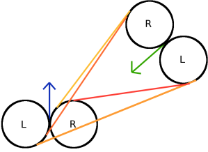
Figure 2. Valid tangent lines

CCC Trajectories

CCC Trajectories are slightly different. They consist of a turn in one direction followed by a turn in the opposite direction, and then another turn in the original direction, like theRLR Trajectory shown in Figure 3. They are only valid when the agent and its goal are relatively close to each other, else one circle would need to have a radius larger than $r_{min}$ , and if we must do that, then theCCC Trajectory is sub-optimal. For the Dubin’s Car there are only 2CCC Trajectories:RLR andLRL. Computing the tangent lines between RR or LL circles won’t help us this time around. The third circle that we turn about is still tangent to the agent and goal turning circles, but these tangent points are not the same as those from tangent line calculations. Therefore, solving these trajectories boils down to correctly computing the location of this third tangent circle.

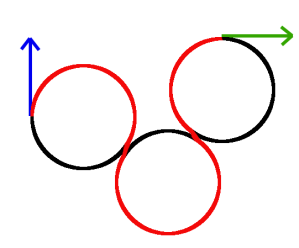
Figure 3. Computing a RLR Trajectory

Tangent Line Construction

In this section, I will discuss the geometry in constructing tangent lines between two circles. First I’ll discuss how to do so geometrically, and then I’ll show how to do so in a more efficient, vector-based manner.

Given: two circles $C_1$ and $C_2$ , with radii $r_1$ and $r_2$ respectively.

Consider the center of $C_1$ as $p_1 = \left(x_1, y_1\right)$ , the center of $C_2$ as $p_2 = \left(x_2, y_2\right)$ , and so on. (Figure 4).

Figure 4. Setup for computing tangents.

Method 1: Geometrically computing tangents

Inner tangents

1. First draw a vector $\vec{V_1}$ from $p_1$ to $p_2$ . $\vec{V_1} = \left(x_2 - x_1, y_2 - y_1\right)$ . This vector has a magnitude:

$D = \sqrt{\left(x_2 - x_1\right)^2 + \left(y_2 - y_1\right)^2}$
2. Construct a circle $C_3$ centered at the midpoint of $\vec{V_1}$ with radius $r_3 = \frac{D}{2}$
That is,

$p_3 = \left(\frac{x_1+x_2}{2}, \frac{y_1+y_2}{2}\right)$

Figure 5. Steps 1 and 2.

3. Construct a circle $C_4$ centered at $C_1$ ’s center, with radius $latex r_4 = r_1 + r_2$

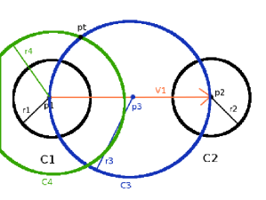
Figure 6. Step 3.

4. Construct a vector $\vec{V_2}$ from $p_1$ to the “top” point, $p_t = \left(x_t, y_t\right)$ of intersection between $C_3$ and $C_4$ . If we can compute this vector, then we can get the first tangent point because $\vec{V_2}$ is pointing at it in addition to $p_t$ . For visual reference, see Figure 7.

Figure 7. Step 4.

5. This is accomplished by first drawing a triangle from $p_1$ to $p_3$ to pt like the one shown in Figure 8. The segments $\overline{p_1p_3}$ and $\overline{p_3p_t}$ have magnitude $r_4 = \frac{D}{2}$ . The segment $\overline{p_1p_t}$ has magnitude $r_3 = r_1 + r_2$ . We are interested in the angle $\gamma = \angle{p_tp_1p_3}$ . $\gamma$ will give us the angle that vector $\vec{V_1}$ that would need to rotate through to point in the same direction as vector $\vec{V_2} = \left(p_t - p_1\right)$ . We obtain the full amount of rotation about the $x$ axis, $\theta$ for $\vec{V_2}$ , by the equation $\theta = \gamma + atan2\left(\vec{V_1}\right)$ (Note: the atan2() function first takes the y-component, and then the x-component) $p_t$ is therefore obtained by traversing $\vec{V_2}$ for a distance of $r_4$ . That is,

$x_t = x_1+\left(r_1+r_2\right)*cos\left(\theta\right)$

$y_t = y_1+\left(r_1+r_2\right)*sin\left(\theta\right)$

Figure 8. Step 5.

6. To find the first inner tangent point pit1 on C1 , we follow a similar procedure to how we obtained pt — we travel along $\vec{V_2}$ from $p_1$ , but we only go a distance of $r_1$ . Because we know $p_t$ , we are now able to actually compute $\vec{V_2} = \left(p_t - p_1\right)$ . Now, we need to normalize $\vec{V_2}$ and
then multiply it by $r_1$ to achieve a vector $latex \vec{V_3}$ to $latex p_{it1}$ from $p_1$ . (Remember that, to normalize a vector, you divide each element by the vector’s magnitude $\to \vec{V_3} = \frac{\vec{V_2}}{\|V_2\|} * r_1$ . $p_{it1}$ follows simply:

$p_{it1} = p_1 + \vec{V_3}$

It may be a bit of an abuse of notation to add a vector to a point, but when we add the components of the point to the components of the vector, we get our new point and everything works out.

7. Now that we have $p_t$ , we can draw a vector $\vec{V_4}$ from $p_t$ to $p_2$ like in Figure 9. Note that this vector is parallel to an inner tangent between $C_1$ and $C_2$

$\vec{V_4} = \left(p_2 - p_t\right)$

We can take advantage of its magnitude and direction to find an inner tangent point on $C_2$ . Given that we’ve already calculated $p_{it1}$ , getting its associated tangent point on $C_2$ , $p_{it2}$ is as easy as:

$p_{it2} = p_{it1} + \vec{V_4}$

Figure 9. Step 7.

I hope this is clear enough for you to be able to compute the other inner tangent point. The trick is to use the “bottom” intersection point between $C_3$ and $C_4$ , and then work everything out exactly the same to get $p_{it3}$ and $p_{it4}$ , which define the other inner tangent line.

Outer tangents

Constructing outer tangents is very similar to constructing the inner tangents. Given the same two circles $C_1$ and $C_2$ as before, and assuming $r_1 \geq r_2$ Remember how we started off by making $C_4$ centered at $p_1$ with radius $r_4 = r_1 + r_2$ ? Well this time around we’ll construct it a bit differently. $C_4$ is centered at $p_1$ as before, but this time it has radius $r_4 = r_1 - r_2$ .

Follow the steps we performed for the interior tangent points, constructing $C_3$ on the midpoint of $\vec{V_1}$ exactly the same as before. Find the intersection between $C_3$ and $C_4$ to get $p_t$ just as before as well. After we’ve gone through all the steps as before up to the point where we’ve obtained $\vec{V_2}$ , we can get the first outer tangent point $p_{ot1}$ by following $\vec{V_2}$ a distance of $r_1$ just as before. I just wanted to note that the magnitude of $\vec{V_2}$ before normalization is $r_4 > r_1$ instead of $r_4 > r_1$ . To get $p_{ot2}$ , the accompanying tangent point on $C_2$ , we perform addition:

$p_{ot2} = p_{ot1} + \vec{V_4}$

This is exactly the same as before. In essence, the only step that changes between calculating outer tangents as opposed to inner tangents is how $C_4$ is constructed; all other steps remains exactly the same.

Method 2: A Vector-based Approach

Now that we understand geometrically how to get tangent lines between two circles, I’ll show you a more efficient way to do so using vectors that has no need for constructing circles $C_3$ or $C_4$ . We didn’t work through the example in the previous section for nothing– we had to work up to Step 7 so that you could have some intuition on why the following vector method works.

1. Draw your circles $C_1$ and $C_2$ as before (Figure 4).
2. Draw vector $\vec{V_1}$ from $p_1$ to $p_2$ . This has magnitude $D$ as before.
3. Draw a vector $\vec{V_2}$ between your tangent points. In this case, it’s easier to start with outer tangent points, which we’ll call pot1 and $p_{ot2}$ . So, $\vec{V_2} = p_{ot2} -p_{ot1}$
4. Draw a unit vector perpendicular to $\vec{V_2}$ . We’ll call it $\hat{n}$ (normal vector).

Figure 10 depicts our setup. In the general case, the radii of $C_1$ and $C_2$ will not be equivalent, but for us it will. This method works for both cases.

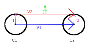
Figure 10. Setup for computing tangents via the vector method

5. Let’s consider some relationships between these vectors.
• The dot product between $\vec{V_2}$ and $\hat{n}$ is 0 because the vectors are perpendicular.
• $\hat{n} \cdot \hat{n} = 1$ because $\hat{n}$ is a unit vector.

• We can modify vector $\vec{V_1}$ to be parallel to $\vec{V_2}$ quite easily by subtraction:

$\vec{V_1} -= \left(r_1-r_2\right) \cdot \hat{n}$

Refer to Figure 10: Setup for computing tangents via the vector method.
Why does this work? For some intuition, consider Step 7 in the previous section: We drew a vector from $p_t$ to $C_2$ ’s center, and
then I stated that the vector was parallel to the vector between the tangent points. Well, both points were equidistant from their
respective tangents; we need to move $p_t$ a distance of $r_2$ to get to the first tangent point. Likewise we need to translate $p_2$ (the center of the other circle) ”down” the same amount of distance.

Using the head-to-tail method of vector addition, you can see that we modified $\vec{V_1}$ to be this same vector! Now that I’ve convinced you that this modification causes $\vec{V_1}$ to be parallel to $\vec{V_2}$ , the following statement holds:

$\hat{n} \cdot \left(\vec{V_1} - \left(\left(r_2-r_1\right) \cdot \hat{n}\right)\right) = 0$

• Simplifying the above equation by distributing $\hat{n}$ :
$\hat{n} \cdot \vec{V_1} + r_1 - r_2 = 0$

• Further simplifying the equation:
$\hat{n} \cdot \vec{V_1} = r_2 - r_1$

• Let’s normalize $\vec{V_1}$ by dividing by its magnitude, $D$ . This doesn’t change the dot product between $\vec{V_1}$ and $\hat{n}$ because the vectors are still perpendicular, but we also have to divide the right-hand side by $D$ :
$\frac{\vec{V_1}}{D} \cdot \hat{n} = \frac{r_2-r_1}{D}$

I’ll refer to the normalized $\vec{V_1}$ Simply as $\hat{V_1}$ from here on.

• Now we can solve for $\hat{n}$ because it is the only unknown in the equations:

• The dot product between two vectors $\vec{A}$ and $\vec{B}$ is defined as:
$\vec{A} \cdot \vec{B} = \|A\|\|B\|cos\left(\theta\right)$
Where $\theta$ is the angle between them. Therefore, in the equation

$\hat{V_1} \cdot \hat{n} = \frac{r_2-r_1}{D}$

$\frac{r_2-r_1}{D}$ is the cosine of the angle between $\hat{V_1}$ and $\hat{n}$ . Because it’s constant, and I don’t want to keep re-typing it, let’s define $c = \frac{r_2-r_1}{D}$ (constant).

• All that remains now is to rotate $\hat{V_1}$ through the angle $acos(c)$ , and it will be equivalent to $\hat{n}$ . Rotating a vector is awell known operation in mathematics.

$\hat{n} = \left(n_x, n_y\right)$ is, therefore:

$n_x = v_{1_x}*c - v_{1_y}*\sqrt{1-c^2}$

$n_y = v_{1_x}*\sqrt{1-c^2} + v_{1_y}*c$

Remember that $c$ is the cosine of the angle between $\hat{V_1}$ and $\hat{n}$ , therefore the sine of the angle is $\sqrt{1-c^2}$ because

$cos^2\left(\theta\right) + sin^2\left(\theta\right) = 1$
6. Knowing $\hat{n}$ as well as $\vec{V_2}$ (remember when we modified $\vec{V_1}$ to be $\parallel$ to $\vec{V_2}$ ?), allows us to very easily calculate the tangent points by first going from the center of $C_1$ along n for a distance of $r_1$ , and then from there following $V_2$ to get the second tangent point.
The other tangent points are easily calculated from this vector-based formalism, and it’s much faster to do than all the geometry transformations
we did with Method 1. Refer to freely available code online for how to actually implement the vector method.

Computing CSC curves

The only reason we needed to compute tangent points between circles is so that we could find the ‘S’ portion of ourCSC curves. Knowing the tangent points on our circles we need to plan to, computingCSC paths simply become a matter of turning on a minimum turning radius until the first tangent point is reached, travelling straight until the second tangent point is reached, and then turning again at a minimum turning radius until the goal configuration is reached. There’s really just one gotcha one needs to worry about this step, and that has to do with the directionality of the circles. When an agent wants to traverse the arc of a circle between two points on the circle’s circumference, it must follow the circle’s direction. That is, an agent cannot turn left (positive) on a right-turn-only (negative) circle. This can become an issue when computing the arc lengths between points on a circle. The thing about all your trigonometry functions is that they will only return you the short angle between things. With directed circles, though, very often you want to actually be traversing the long angle between two
points on the circle. Fortunately there is a simple fix.

Computing Arc Lengths

Given: A circle $C_1$ centered at $p_1$ with points $p_2$ and $p_3$ along its circumference, radius $r_1$ , and circle directionality $d$ , which can be “left” or “right”.

Arc lengths of circles are computed by multiplying the radius of the circle by the angle $\theta$ between the points along the circumference. Therefore arc length, $L = r_1 * \theta$ , and $\theta$ can be naively computed using the law of cosines
after you compute the Euclidean distance between the points. I say naively because this method will only give you the shorter arc length, which will not always be correct for your directed circles (Figure 11).

Figure 11. A scenario where the arc length on a directed circle is actually the larger of the two between the points.

A better strategy would be to generate vectors from the center of the circle to the points along the circumference. That is, $\vec{V_1} = p_2 - p_1$ and $\vec{V_2} = p_3 - p_1$ . Let’s assume that the arc you want to traverse is from $p_2$ to $p_3$ with direction $d$ .

We can use the $atan2()$ function to compute the small angle between the points as before, but the difference is that $atan2()$ gives us directional information. That is, $\theta = atan2\left(\vec{V_3}\right) - atan2\left(\vec{V_2}\right)$ will be positive or negative depending on what direction $\vec{V_1}$ rotated to end up at $\vec{V_2}$ . A positive rotation is a “left” turn and a negative rotation is a “right” turn. We can check the sign of this angle against $d$ . If our angle’s sign disagrees with the direction we’d like to turn, we’ll correct it by either adding or subtracting 2 $\pi$ .

That is:

With a function like this to compute your arc lengths, you will now very easily be able to compute the duration of time to apply your “turn left” or “turn right” controls within a circle.

The geometry of CSC trajectories

RSR, LSL, RSL, and LSR trajectories are all calculated similarly to each other, so I’ll only describe theRSR trajectory (Figure 12).

Given starting configuration $s = {x_1, y_1,\theta_1}$ and goal configuration $g = {x_2, y_2, \theta_2}$ , we wish to compute a trajectory that consists of first turning right (negative) at a minimum turning radius, driving straight, and then turning right (negative) again at minimum turning radius until the goal configuration is reached. Assume that the minimum turning radius is $r_min$ .

First, we must calculate the circles about which the agent will turn — a circle of minimum radius $C_1$ to the “right” of s as well as a circle of minimum radius $C_2$ to the “right” of $g$ . The center of $C_1$ , becomes
$p_{c1} = \left(x_1 + r_{min}*cos\left(\theta_1-\frac{\pi}{2}\right), y_1 + r_{min}*sin\left(\theta_1-\frac{\pi}{2}\right)\right)$

Similarly, the center of $C_2$ becomes

$p_{c2} = \left(x_2 + r_{min}*cos\left(\theta_2-\frac{\pi}{2}\right), y_1 + r_{min}*sin\left(\theta_2-\frac{\pi}{2}\right)\right)$

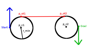
Figure 12. Using what we’ve learned to compute a RSR Trajectory

Now that we’ve obtained the circles about which the agent will turn, we need to find the outer tangent points we can traverse. I demonstrated earlier how one would go about calculating all the tangent points given two circles. For an RR circle, though, only one set of outer tangents is valid. If you implement your tangent-pt computing function appropriately, it will always return tangent points in a reliable manner. At this point, I’ll assume you are able to obtain the proper tangent points for a right-circle to right-circle connection.

Your tangent point function should return points $p_{ot1}$ and $p_{ot2}$ which respectively define the appropriate tangent points on $C_1$ , the agent’s right-turn circle and $C_2$ , the query configurations’ right-turn circle.

Now that we’ve calculated geometrically the points we need to travel through, we need to transform them into a control the agent can understand. Such a control should be in the form of “do this action at this timestep”. For the Dubin’s car, this is pretty easy. If we define a control as a pair of (steering angle, timesteps), then we can define a RSR trajectory as an array of 3 controls: ( $-steeringMax$ , $timesteps1$ ), ( $0$ , $timesteps2$ ), and ( $-steeringMax$ , $timesteps3$ ). We still need to compute the number of timesteps, but this isn’t so bad.

We know ( $x_1,y_1$ ) , the position of our starting configuration, as well as $p_{ot1}$ our outer tangent point. Both of these points lie on the circumference of the minimum turning-radius “right-turn only” circle to the right of the $s$ , the starting configuration. Now we can take advantage of our ArcLength function to compute the distance between the two points given a right-turn. Typically, simulations don’t update entire seconds at once, but rather some some $\delta$ . This is a type of integration calledEuler integration that allows us to closely approximate the actual trajectory the car should follow, though not perfectly so. Because we’ve defined the Dubin’s car’s update function as a linear function of the form

$\dot{x} =cos\left(\theta\right)$

$\dot{y} = sin\left(\theta\right)$

$\dot{\theta} = \frac{1}{r_{turn}}$
then we actually travel in a straight line from timestep to timestep. A big $\delta$ therefore results in a poor approximation of reality. As $\delta$ approaches 0, though, we more closely approximate reality. Typically a delta in the range of [0.01,0.05] is appropriate, but you may need finer or coarser control. Accounting for $\delta$ , our update equations become:

$x_{new} = x_{prev} + \delta*cos\left(\theta\right)$

$y_{new} = y_{prev} + \delta*sin\left(\theta\right)$

$\theta_{new} = \theta_{prev} + \frac{\delta}{r_{turn}}$
Now that we have decided on a value for $\delta$ , we can compute the number of timesteps to apply each steering angle. Given the length of an arc $L$ (computed using the ArcLength function, or just simply the magnitude of the tangent line)

$timesteps_x = \frac{L}{\delta}$

Computing the other trajectories now becomes a matter or getting the right tangent points to plan towards. TheRSR andLSL trajectories will use outer tangents while theRSL andLSR trajectories use the inner tangents.

Computing CCC trajectories

Two of the Dubin’s shortest paths don’t use the tangent lines at all. These are theRLR andLRL trajectories, which consist of three tangential, minimum radius turning circles. Very often, these trajectories aren’t even valid because of the small proximity that $s$ and $g$ must be to each other for such an arrangement of the three circles to be possible. If the distance between the agent and query configurations’ turning circles is less than $4r_{min}$ , then aCCC curve is valid. I say less than $4r_{min}$ , because if the distance were equal, then aCSC trajectory is more optimal.

For CCC trajectories, we must calculate the location of the third circle, as well as its tangent points to the circles near s and g. To be more concrete, I’ll address theLRL case, shown in Figure 13.

Consider the minimum-radius turning circle to the “left” of $s$ to be $C_1$ and the minimum-radius turning circle to the “left” of $g$ to be to $C_2$ . Our task is now to compute $C_3$ , a minimum-radius turning circle tangent to both $C_1$ and $C_2$ plus the points $p_{t1}$ and $p_{t2}$ which are respective points of intersection between $C_1$ and $C_3$ , and between $C_2$ and $C_3$ . Let $p_1, p_2, p_3$ be the centers of $C_1, C_2,$ and $C_3$ , respectively. We can form the triangle $\bigtriangleup{p_1, p_2, p_3}$ using these points. Because $C_3$ is tangent to both $C_1$ and $C_2$ , we already know the lengths of all three sides.

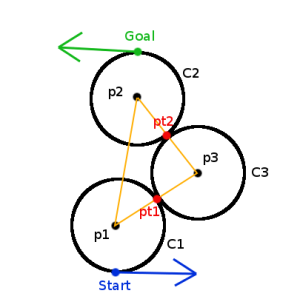
Figure 13. Computing LRL trajectory

Segments $\overline{p_1p_3}$ and $\overline{p_2p_3}$ have length $2r_{min}$ and segment $\overline{p_1p_2}$ has length $D = \sqrt{\left(x_2 - x_1\right)^2 + \left(y_2 - y_1\right)^2}$ . We are interested in the angle $\theta = \angle{p_2p_1p_3}$ because that is the angle that the line between $C_1$ and $C_2$ ( $\vec{V_1} = p_2 - p_1$ ) must rotate to face the center of $C_3$ , which will allow us to calculate $p_3$ . Using the law of cosines, we can determine that $\theta = cos^{-1}\left(\frac{D}{4r_min}\right)$

In a LRL trajectory, we’re interested in a $C_3$ that is “left” of $C_1$ . At the moment, we have an angle, $\theta$ that represents the amount of rotation that vector $\vec{V_1} = \left(p_2 - p_1\right)$ must rotate to point at the center of $C_3$ . However, $\theta$ ’s value is only valid if $\vec{V_1}$ is parallel to the x-axis. Otherwise, we need to account for the amount $\vec{V_1}$ is rotated with the $atan2\left(\right)$ function — $atan2\left(\vec{V_1}\right)$ . For aLRL trajectory, we want to add $\theta$ to this value, but for anRLR trajectory we want to subtract $\theta$ from it to obtain a circle “to the
right” of $C_1$ . (Remember that we consider left, or counter-clockwise turns to be positive.)

Now that theta represents the absolute amount of rotation, we can compute

$p_3 = \left(x_1 + 2r_{min}cos\left(\theta\right), y_1 + 2r_{min}sin\left(\theta\right)\right)$

Computing the tangent points $p_{t1}$ and $p_{t2}$ becomes easy; we can define vectors from the $p_3$ to $p_1$ and $p_2$ , and walk down them a distance of $r_{min}$ . As an example, I’ll calculate $p_{t1}$ . First, obtain the vector $\vec{V_2}$ from $p_3$ to $p_1$ ; $\vec{V_2} = p_1 - p_3$ . Next, change the vector’s magnitude to $r_{min}$ by normalizing it and multiplying by $r_{min}$ (or just dividing its components by 2, as its magnitude should already be $2r_{min}$ ).
$\vec{V_2} = \frac{\vec{V_2}}{\|V_2\|} * r_{min}$

Next, compute $p_{t1}$ using the new $\vec{V_2}$ ;
$p_{t1} = p_3 + \vec{V_2}$

Computing $p_{t2}$ follows a similar procedure. At this point we have everything we need for ourCCC trajectory! We have three arcs as before, from $\left(x_1, y_1\right)$ to $p_{t1}$ . From $p_{t1}$ to $p_{t2}$ , and from $p_{t2}$ to $\left(x_2, y_2\right)$ . One can compute arc lengths and durations as before to finish things off.

Conclusions

So now that we’ve computed all of the shortest paths for the Dubin’s Car, what can we do next? Well, you could use them to write a car simulator. The paths are very quick to compute, but are what’s known as ”open-loop” trajectories. An open-loop trajectory is only valid if you apply the desired controls exactly as stated – so a computer. Even if you used a computer to control your car, this would still only work perfectly in simulation. In the real-world we have all kinds of sources for error, that we represent as uncertainty in our controls. If a human driver tried to apply our Dubin’s shortest path controls, they wouldn’t end up exactly on target, would they? Perhaps in a later article I will discuss motion planning under uncertainty, but for now I defer you to the internet.

Another application we could use these shortest path calculations for would be something known as a rapidly exploring random tree, orRRT. An RRT uses the know-how of planning between two points to find reachable points in an environment that has obstacles. The resulting structure of points that are connected is a tree with a root at our start, and the paths one gets from the tree can look pretty good; imagine a car deftly maneuvering around things in its way. RRTs are a big topic of research right now, and Steven LaValle has a wealth of information about them.

Following from the Dubin’s RRT idea, you might one day use a much more complicated car-like robot. For this complicated car-like robot you may want to also use an RRT. Remember when I said that the resulting structure of an RRT looks like a tree with its root at our start? Well, to ”grow” this tree, one has to continue adding points to it, and part of that process is determining which point in the tree to connect to. Typically this is done by just choosing the closest point in the tree. ”Closest” usually means, ”the shortest line between myself and any point in the tree”. For a lot of robots (holonomic especially), this straight-line distance is just fine, but for car-like (nonholonomic) robots it may not be good enough, because you can’t always move on a straight line between start and goal. Therefore, you could use the length of the Dubin’s shortest path instead of the straight-line shortest path as your measure of distance! (We’re using the Dubin’s shortest paths as a ”distance metric”).

In reality, the Dubin’s shortest paths are not a true distance metric because they are not ”symmetric”, which means that the distance from A to B isn’t always the same as the distance from B to A. Because the Dubin’s car can only move forward, it isn’t symmetric. However, if you expanded the Dubin’s car to be able to move backwards, you’d have created aReeds-Shepp car, and the Reeds-Shepp shortest paths are symmetric.

Acknowledgement:

I’d like to thank my colleague Jory Denny for LaTeX sorcery and various grammar edits.

I’ve made the code (sans graphics stuff) available on my GitHub account: https://github.com/gieseanw/Dubins

查看全文
如若内容造成侵权/违法违规/事实不符，请联系编程学习网邮箱：809451989@qq.com进行投诉反馈，一经查实，立即删除！

做双眼皮后脸中间长
...
2024/4/28 16:07:01
做双眼皮后脸比例变了
...
2024/4/28 0:47:13
2017年暑期前端开发实习-阿里内推一面
1. 自我介绍 2. 项目介绍 3. CSS 1）介绍一下css盒模型盒模型基本成了面试必问的问题，有W3C的盒模型和IE浏览器下的盒模型，盒模型从外到里包括：margin、border、padding、content。 （1）W3C盒模型的宽度 co…...
2024/4/21 14:57:47
新手配置vim
原文地址：http://blog.sina.com.cn/s/blog_5ca785c30100dk6x.html Vim很好很完美是公认的了，但是对新手来说，上手毕竟不是很容易。Windows下程序员很多都很喜欢Source Insight这个工具来看代码，各种语法高亮看着很舒服。vim作为为程序员打造的编辑器，没有道理不可以通过配…...
2024/4/20 16:01:32
iptTable规范
规范之HTML 先在当前页面放入几个表格设置按钮的html（样式可能需重新调整） <div class"bottom_nav1 ta_l" style"padding: 0;height: 32px;width: 300px;margin:4px auto 0;"><a class"qxfp" ng-click"addR…...
2024/4/21 14:57:45
在计算机术语中英文cad是指,CAD中英语词汇及命令大全
CAD中英语词汇及命令大全对于从事CAD相关职业的朋友来说，加深认识CAD中英语词汇及命令是很有必要的，今天小编特意整理了这些东西，希望对大家有帮助!2D Solid 二维实体 2D 实面2D Wireframe 二维线框3D Array 三维阵列 3D 阵列3D Dynamic View…...
2024/4/25 10:04:31
做做双眼皮后多久能要孩子吗
...
2024/4/28 12:40:16
settings PreferenceActivity网博收录
《SharedPreferences和PreferenceActivity》《Android之PreferenceActivity》《在Android中Preferences数据存储的使用》《Android的设置界面及Preference使用》《OnPreferenceChangeListener分析，以及与OnPreferenceClickListener的区别》《使用PreferenceActivity时，如…...
2024/4/28 16:51:55
做双眼皮过程视频
...
2024/4/20 15:10:20
做双眼皮感觉脸变大了
...
2024/4/24 0:25:29
做做双眼皮多久能修复
...
2024/4/19 17:12:35
整理学习：100多道前端面试题（一起加油，且行且珍惜）
前言当你准备去面试时，你不妨看一些面试的题目（推荐掘金）来提醒自己究竟掌握得怎么样，比如题目笔者最近一边写项目，一边整理前端面试题，打算完成项目就差不多去实习了… 没有特别宏大的目标&#xf…...
2024/4/21 14:57:43
做双眼皮多久能上班
...
2024/4/21 14:57:41
做双眼皮多久能化眼妆
...
2024/4/21 14:57:41
极致 Web 性能 —— SPA 性能优化
前言前端框架时代，为开发体验、效率与页面性能带来，非常大的革命。大家纷纷拿起一系列打包工具(webpack/parcel etc.)，配合一系列加载器快速搭建起一个 SPA 页面。 SPA 应用带来的好处非常明显； 提升页面切换体验降低切换时间易…...
2024/4/21 14:57:40
做双眼皮多久能抽烟
...
2024/4/21 14:57:39
做双眼皮多久可以抽烟
...
2024/4/23 15:52:41
做双眼皮的专业知识
...
2024/4/22 19:49:11
做双眼皮的男生
...
2024/4/21 14:57:37
做双眼皮的目的
...
2024/4/21 14:57:34